all Think Trillion Story
Think Trillion :: ‘Trillion Dollar Economy’/ ‘Trillion Dollar Company/Market/Potential’/ ‘Trillion Dollar Country’ or anything that implies the big figure ‘Trillion‘
Portray All Stories ON ‘Trillion Dollar Economy’/ ‘Trillion Dollar Company/Market’/ ‘Trillion Dollar Country’ or anything that implies the big figure ‘Trillion‘ as ‘Think Trillion Story’ here.
Add Story/ Your Say
[*Select Category/Tag: Think Trillion at Your Next Publish Screen.]
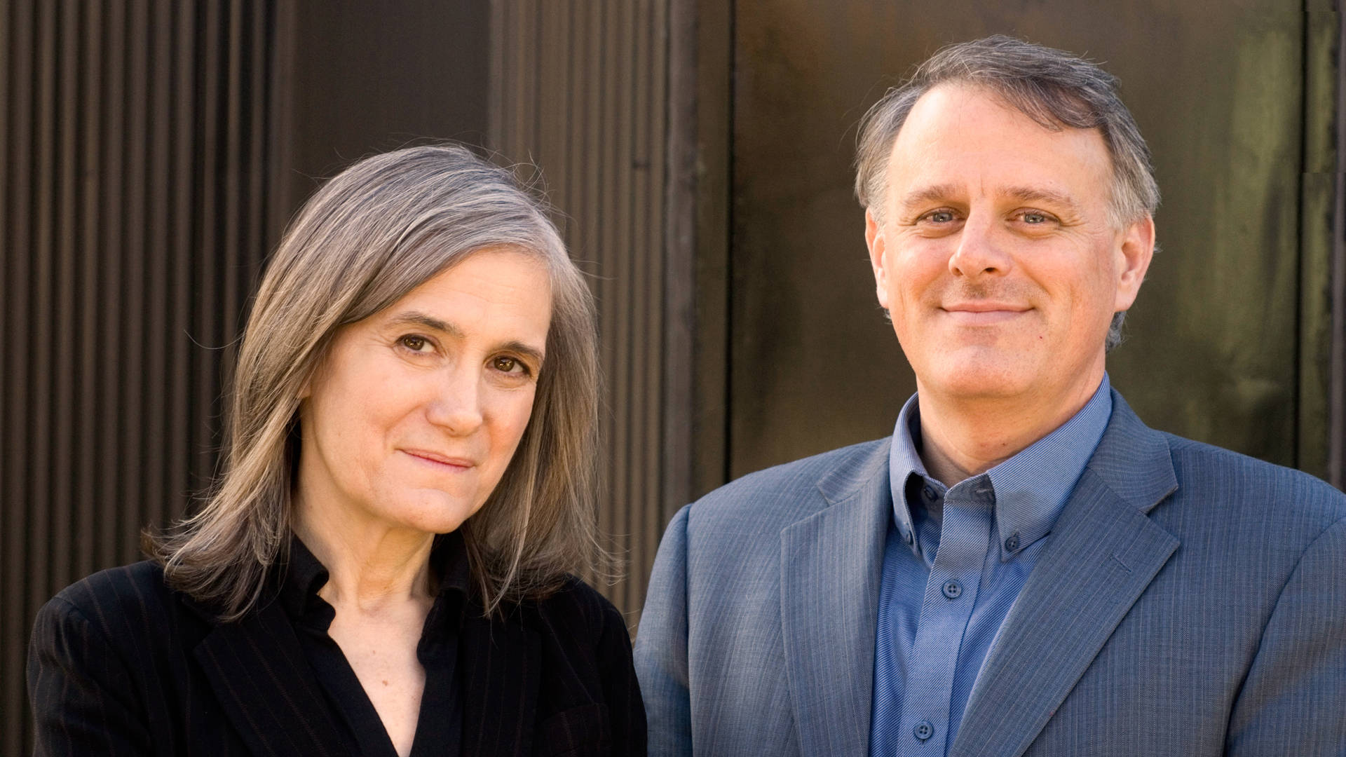
Obama’s Trillion-Dollar Nuclear-Arms Train Wreck
By Amy Goodman & Denis Moynihan
STANFORD, Calif.—“Now I am become Death, the destroyer of worlds.” These were the words from the Hindu religious text, the Bhagavad-Gita, that flashed through the mind of the man credited with creating the first atomic bomb, J. Robert Oppenheimer, as the first nuclear explosion in history lit up the dark desert sky at the Trinity blast site in New Mexico on July 16, 1945.
Weeks after that, the atomic bombing of Hiroshima, then Nagasaki, killed hundreds of thousands of civilians, and thrust the world into the atomic age. Since then, humanity has lived with the terrible prospect of nuclear war and mass annihilation. Conventional wisdom holds that the likelihood that these unconventional weapons will be used has decreased since the end of the so-called Cold War. That perception has been challenged lately, especially since President Barack Obama announced a 30-year, $1 trillion program to modernize the U.S. nuclear-weapon arsenal.
Secretary of State John Kerry visited the Hiroshima Peace Memorial Museum on Monday, the first sitting U.S. secretary of state to visit the site. Kerry was in Japan for a meeting of the G-7 nations. In his public remarks at the memorial, Kerry offered no apology for the nuclear attacks. He did say, though, that the museum “was a reminder of the depth of obligation that every single one of us in public life carries—in fact, every person in position of responsibility carries—to work for peace … to create and pursue a world free from nuclear weapons.”
Despite the lofty rhetoric, President Obama has launched what the Alliance for Nuclear Accountability calls the “Trillion Dollar Trainwreck.” That is the title of a new report on Obama’s massive plan to modernize the U.S. nuclear-weapons arsenal, to be released next Monday. Marylia Kelley is one of the report’s authors. She serves as executive director of Tri-Valley CAREs, or Communities Against a Radioactive Environment, a partner organization with the Alliance. Of Kerry’s visit to Hiroshima, Kelley said, on the “Democracy Now!” news hour, “Kerry went empty-handed. The United States needs to go with a concrete plan to roll back its own nuclear-weapons program. You cannot preach abstinence, in terms of nuclear weapons, from the biggest bar stool in the room.”
“The United States is initiating a new nuclear arms race, because the other nuclear-armed states, of course, when they look at our ‘modernization program,’ are now beginning their own,” she told us. “We need this to be rolled back.” Kelley lives in Livermore, California, home to one of the U.S. government’s national laboratories dedicated to developing and manufacturing nuclear bombs.
President Obama delivered his first address on the U.S. nuclear arsenal on April 5, 2009, in Prague: “Today, the Cold War has disappeared but thousands of those weapons have not. In a strange turn of history, the threat of global nuclear war has gone down, but the risk of a nuclear attack has gone up. More nations have acquired these weapons. Testing has continued. Black-market trade in nuclear secrets and nuclear materials abound,” he said.
As with his pledge to close the U.S. prison at Guantanamo Bay, his pledge to move the U.S. toward nuclear disarmament seems to have been abandoned. Grass-roots groups in the Alliance for Nuclear Accountability would like to see Obama make an historic trip to Hiroshima, as the first sitting U.S. president to do so. “If Obama goes to Hiroshima,” Marylia Kelley said, “he needs to use that as an opportunity, not to speak empty promises and rhetoric about an eventual world free of nuclear weapons, but to make concrete proposals about how the United States is going to take steps in that direction and how we’re going to change course, because right now we’re taking giant steps in the opposite direction.”
The U.S. nuclear arsenal, and all the expense, nuclear waste and immense danger it continuously poses, has received almost no attention in the U.S. presidential debates. The day after he launched his campaign in late May 2015, Sen. Bernie Sanders was asked about the trillion-dollar nuclear-arsenal upgrade at a town hall in New Hampshire. “What all of this is about is our national priorities,” he replied. “Who are we as a people? Does Congress listen to the military-industrial complex, who has never seen a war that they didn’t like? Or do we listen to the people of this country who are hurting?”
In 1946, the year after Trinity, after Hiroshima and Nagasaki, Albert Einstein, whose theory of relativity gave birth to the atomic bomb, offered a warning to the world that remains starkly relevant today: “The unleashed power of the atom has changed everything save our modes of thinking and we thus drift toward unparalleled catastrophe.”
as per our monitoring this Story originally appeared * : ) here → *
Obama’s Trillion-Dollar Nuclear-Arms Train Wreck

Trillion Dollar Design
Welcome to the website of Trillion Dollar Design, LLC. We hand-craft championship belts for all occasions. Contact us to order your Championship Belt today.

Dashielle Mayfield (August 26, 2006 – May 10, 2020) Non-Violent Champion Cat. We are thankful for the best 13 years ever living with you!!! RIP our lovables. Gone too soon…

Don’t be defiant, believe science. Wear your mask and life will last.
September 2020

Trillion Dollar Design, LLC Welcomes Trevor Clymens 2016 and 2018 Champion B-Modified Antioch Speedway – Bridging the Gap for Non-Violent Championship Belts June 20, 2020
Supporters of Non-Violent Champions Tony Rock and Tony Mayfield
John Witherspoon supports Tony Mayfield non-violent champion

Non-Violent Comedy Legend spent his valuable time with me on September 14, 2019. His last words he shared with me about his non-violent laughter for all to enjoy. RIP John Witherspoon October 29, 2019. PS: Deep appreciation

Special thanks to Cedric the Entertainer for accepting non-violent champion belt.

Ice Cube with the Non-Violent Championship Belt on the set of First Take. Special thanks.

Tony Mayfield Non-Violent Champion For Life

Non-violent champion Tony Mayfield goes to the Big 3 Championship at the Staples Center

After practice Stephen Jackson takes time out for non-violent champion Tony Mayfield

From the movie “The Wash” Tray Deee and non-violent champion Tony Mayfield

Special Thanks to Michael Rappaport

Non-violent champion Tony Mayfield makes appearance on the set of First Take

Non-Violent Championship Belts – Tony Mayfield, Designer

MC Hammer and Designer Tony Mayfield on the set of First Take

1974-1975 NBA Champion Living Legend Al Attles

Rick Welts, President, Holds Golden State Warriors 3X World Championship Belt
Designer Tony Mayfield
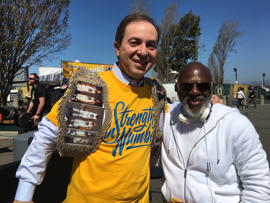
Warriors’ Owner Loves Trillion Dollar Design, LLC, Non-Violent Championship Belts

Warriors Hall of Famer Chris Mullin


Welcome Harry Davis of Gucci San Francisco to the Non-Violent Champions
Designer Tony Mayfield
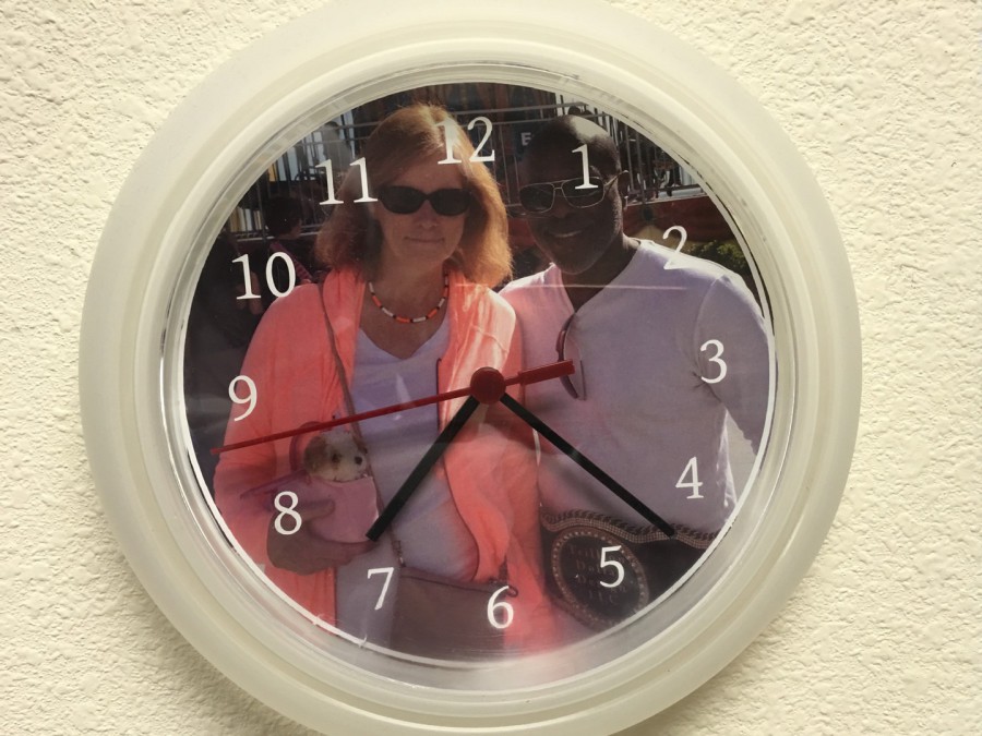
Trillion Dollar Design, LLC, custom-made photo clocks. Contact us to order your personalized lifetime memory.

First Take Sports Analyst Max and Tony Mayfield after the show

First Take Championship Belt

Say it loud: Charlie Murphy!!!! Last appearance with him.
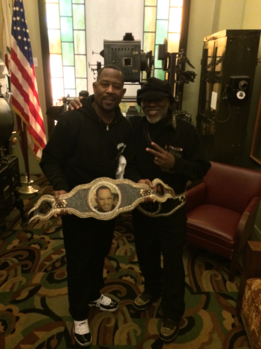
Special Thanks to Martin Lawrence

Special Thanks to Damon Wayans

Special Thanks to Marlon Wayans

Special Thanks to Sommore

Soulful R&B Singer Freddie Jackson
Thank you for visting our site.
as per our monitoring this Story originally appeared * : ) here → *
Trillion Dollar Design
5G Market are Going From $31 Billion in 2020 to $11 Trillion by 2026, Research Report by ReportsnReports
PUNE, India, Nov. 13, 2019 /PRNewswire/ — The 2019 study has 246 pages, 121 tables and figures. The leading vendors in the 5G market have invested in high-quality technology and processes to develop leading edge monitoring and digital triggering activation capability. 5G is the most disruptive force seen in centuries. 5G Market are going from $31 billion in 2020 to $11 trillion by 2026. It has more far reaching effect than a stronger military, than technology, than anything.
5G markets encompass virtualization, cloud, edge, and functional splits. As 5G networks come on line in 2020, they require increasing sophistication from mobile operators. The challenge going forward in mobile network buildout is to bring together a growing number of LTE and 5G radio access technologies. A range of connectivity services are needed. APIs are needed in each small cell to manage connectivity to a number of customer sensors that are implemented in different segments.
Get Free Sample Copy of 5G Market Research Report at https://www.reportsnreports.com/contacts/requestsample.aspx?name=2680586
The 5G sales at $31.3 billion in 2020 are forecast to reach $11.2 trillion in 2026. Networks spending has been transformed from macro cell tower dominance to 80% of spending on infrastructure and equipment for 5G. 5G supports wireless communications across short distances. All the indoor and outdoor places need to increase wireless coverage, providing significant market growth for 5G.
The digital economy, self-driving cars, drones, smart traffic lights, and smart connectivity of sensor enabled edge devices need more wireless coverage. According to Susan Eustis, leader of the team that prepared the research, “5G suppliers have a focus on broadband improvement. Power and performance are being improved. 5G improves the transmission coverage and density.”
This 5G coverage is needed as IoT, the Internet of things and smart phone video increase transmission needs.
Get Discount on this Research Report at https://www.reportsnreports.com/contacts/discount.aspx?name=2680586
Companies Profiled
Market Leaders:
Intel
Ericsson
Huawei
Nokia / Alcatel-Lucent
NEC
Qualcomm
Samsung
Fujitsu
ip.access
Market Participants:
ADT Inc
Advantech Co Ltd
Alphabet / Google
Amazon.com (AMZN)
AMS ag
Apple
AT&T
Baidu (BIDU)
BlueShift Memory
Broadcom
Cisco
Crown Castle (CCI)
Cypress Semiconductor
Dexcom Inc
Ericsson
Facebook (FB)
Garmin ltd
Huawei
IBM
IBM / Red Hat
Intel
Juniper Networks
Kensaq.com
Amazon
Netflix
Marvell Technology Group
Mavenir
Mellanox Technologies
Micron
Microsoft (MSFT)
NeoPhotonics 400G CFP8 PAM
Nokia
Nvidia Speeds and Feed
Qualcomm
Qorvo
Rackspace
Rogers Communications
Salesforce (CRM)
Samsung
Sensata Technology
Silicon Laboratories
Skyworks Solutions
SoftBank
Telus
Tencent (TCEHY)
Tesla
Toyota and Panasonic
Tsinghua
Twilio
Verizon
Xilinx
Direct Purchase of 5G Market, Extending Human Eyesight, Extending Human Senses Forecasts, Worldwide, 2020 to 2026 Report at https://www.reportsnreports.com/purchase.aspx?name=2680586
Table of Contents:
5G Executive Summary
- 5G Market Description and Market Dynamics
- 5G Market Leaders and Forecasts
- 5G Market Analysis
- 5G Research and Technology
- 5G Company Profiles
Another Related Research Report The Private LTE & 5G Network Ecosystem: 2020 – 2030 – Opportunities, Challenges, Strategies, Industry Verticals & Forecasts – Report presents an in-depth assessment of the private LTE and 5G network ecosystem including market drivers, challenges, enabling technologies, vertical market opportunities, applications, key trends, standardization, spectrum availability/allocation, regulatory landscape, deployment case studies, opportunities, future roadmap, value chain, ecosystem player profiles and strategies. The report also presents forecasts for private LTE and 5G network infrastructure investments from 2020 till 2030. The forecasts cover three submarkets, two air interface technologies, 10 vertical markets and six regions.
Expected to reach $4.7 Billion in annual spending by the end of 2020, private LTE and 5G networks are increasingly becoming the preferred approach to deliver wireless connectivity for critical communications, industrial IoT, enterprise & campus environments, and public venues. The market will further grow at a CAGR of 19% between 2020 and 2023, eventually accounting for nearly $8 Billion by the end of 2023. Order a Copy of this Research Report at https://www.reportsnreports.com/purchase.aspx?name=2640367
About Us:
ReportsnReports.com is your single source for all market research needs. Our database includes 100,000+ market research reports from over 95 leading global publishers & in-depth market research studies of over 5000 micro markets. With comprehensive information about the publishers and the industries for which they publish market research reports, we help you in your purchase decision by mapping your information needs with our huge collection of reports. We provide 24/7 online and offline support to our customers.
Contact:
Vishal Kalra
Tower B5, office 101,
Magarpatta SEZ,
Hadapsar, Pune-411013, India
+1-888-391-5441
[email protected]
Connect With Us on:
Facebook: https://www.facebook.com/ReportsnReports/
LinkedIn: https://www.linkedin.com/company/reportsnreports
Twitter: https://twitter.com/marketsreports
RSS/Feeds: http://www.reportsnreports.com/feed/l-latestreports.xml
SOURCE ReportsnReports

as per our monitoring this Story originally appeared * : ) here → *
5G Market are Going From $31 Billion in 2020 to $11 Trillion by 2026, Research Report by ReportsnReports

Mitch McConnell Blames the Poor for Trump’s Trillion-Dollar Deficit
In a life filled with uncertainty, there are a few things you can always count on. First, that death comes for everyone. Second, that the current president of the United States will call an adult-film star he paid to keep quiet about an alleged affair “horseface” on social media. And third, that after passing a $1.5 trillion tax cut they insisted would pay for itself and then some, Republicans would blame social services like Medicare, Medicaid, and Social Security for exploding deficits and debt and insist that such “entitlements,” sadly, have got to go.
As a reminder, the Grand Old Party put on a big show of pretending to care about “fiscal responsibility” when Barack Obama was in office and mouth-watering tax cuts weren’t on the line. “Only one thing can save this country, and that’s to get a handle on this deficit-and-debt issue,” Majority Leader Mitch McConnell insisted after the 44th president won his second term. “The federal fiscal burden threatens the security, liberty, and independence of our nation,” the Republican Party platform warned in 2016. “You’re bankrupting our grandchildren!” was a common refrain, as were proclamations such as, “I won’t endorse a bill that adds one penny to the deficit!” Then Donald Trump won the election, and all those worries about crippling the next generation and the country going to hell in a handbasket vanished overnight—almost as though it was feigned in the first place!—with Republicans not only demanding that Congress pass a deficit-busting piece of legislation so that the president and his children could pay even fewer taxes than they already do, but maintaining—laws of math, physics, time and space be damned—that the bill once known as the “Cut Cut Cut Act” would actually help shrink the deficit.
But as the G.O.P. surely knew, that was never going to happen. Instead, as we learned this week, the U.S. budget deficit increased to $779 billion for the fiscal year, a 17 percent increase from the year prior, which is extra bad considering the economy is doing well, a scenario in which the federal deficit typically falls. Luckily, Mitch McConnell knows exactly who and what to blame:
“It’s disappointing, but it’s not a Republican problem,” McConnell said Tuesday in an interview with Bloomberg News when asked about the rising deficits and debt. “It’s a bipartisan problem: unwillingness to address the real drivers of the debt by doing anything to adjust those programs to the demographics of America in the future.”
The “real” drivers of debt, according to McConnell, are “Medicare, Social Security, and Medicaid,” “entitlements” from which the Senate majority leader would cut off the old and poor if only he could get Democrats to sign on. (That’s probably unlikely to happen, given Nancy Pelosi’s statement today that, “Like clockwork, Republicans in Congress are setting in motion their plan to destroy the Medicare, Medicaid, and Social Security that seniors and families rely on, just months after they exploded the deficit by $2 trillion with their tax scam for the rich,” and Chuck Schumer’s that suggesting cuts to “middle-class programs like Medicare, Social Security, and Medicaid as the only fiscally responsible solution to solve the debt problem is nothing short of gaslighting.”)
McConnell’s take on the situation echoes that of the White House, whose National Economic Council director, Larry Kudlow, said last month that he doesn’t “buy” the argument that tax cuts increase the deficit, and that the real problem is “principally spending too much.” (Kudlow, who has a penchant for never being right about anything, also claimed in June that the deficit was “coming down rapidly.”) Treasury Secretary Steven Mnuchin was even more blunt while telling his assessment to CNN last week, “People are going to want to say the deficit is because of the tax cuts. That’s not the real story.” (The report out of his own department suggests otherwise.) Incidentally, in June, reports circulated that the Trump administration was trying to figure out a workaround to cut another $100 billion from the tax bills of the wealthiest Americans, and in late September, House Republicans passed a piece of legislation that would add more than $600 billion to the debt over the next decade. Neither measure will come to fruition, but on the off-chance that one does, we’re sure McConnell stands ready to blame the poor and elderly freeloaders who clearly hate America.
If you would like to receive the Levin Report in your inbox daily, click here to subscribe.
as per our monitoring this Story originally appeared * : ) here → *
Mitch McConnell Blames the Poor for Trump’s Trillion-Dollar Deficit
The Nonprofit Sector in Brief 2018
12.13.2018
Brice McKeever
- ######
- #Background Setup
- ######
- library(httr)
- library(tidyverse)
- library(stringr)
- library(RCurl)
- library(reshape2)
- library(RColorBrewer)
- library(extrafont)
- library(knitr)
- library(foreign)
- library(kableExtra)
- library(urbnthemes)
- library(grid)
- library(gridExtra)
- #set_urban_defaults()
- set_urban_defaults()
- ######
- #Download Raw NCCS Data
- ######
- #This code will use the following NCCS data sets, so import separately using defined functions, and save in the “Data” folder
- #Retrieve NCCS Data Archive download functions
- source(“NCCS_Code/Prep IRS BMF.R”)
- source(“NCCS_Code/Prep NCCS Core File.R”)
- #The following code will retrieve the stated data sets from the NCCS Data Archive.
- #This code is commented out in final to avoid repeated (and bandwidth intensive) downloads
- #IRS Business Master Files:
- #bm0601
- #bm0601 <- getbmffile("2006", "01")
- ##bm1106
- #bm1106 <- getbmffile("2011", "06")
- ##bm1502
- #bm1502 <- getbmffile("2015", "02")
- ##bm1602
- #bm1602 <- getbmffile("2016", "02")
- ##
- ##core2005pf
- #core2005pf <- getcorefile(2005, "pf")
- ##core2005pc
- #core2005pc <- getcorefile(2005, "pc")
- ##core2005co
- #core2005co <- getcorefile(2005, "co")
- #
- ##
- ##core2010pf
- #core2010pf <- getcorefile(2010, "pf")
- ##core2010pc
- #core2010pc <- getcorefile(2010, "pc")
- ##core2010co
- #core2010co <- getcorefile(2010, "co")
- #
- ##
- ##core2014pf
- #core2014pf <- getcorefile(2014, "pf")
- ##core2014pc
- #core2014pc <- getcorefile(2014, "pc")
- ##core2014co
- #core2014co <- getcorefile(2014, "co")
- #
- ##
- ##core2015pf
- #core2015pf <- getcorefile(2015, "pf")
- ##core2015pc
- #core2015pc <- getcorefile(2015, "pc")
- ##core2015co
- #core2015co <- getcorefile(2015, "co")
- ######
- #Import Index Tables
- ######
- #The NTEE Lookup file can be downloaded from: http://nccs-data.urban.org/data/misc/nccs.nteedocAllEins.csv
- #The following code assumes that it has been saved in the local “Data” folder
- #retrieve from CSV:
- nteedocalleins <- read_csv("Data/nteedocalleins.csv",
- col_types = cols_only(EIN = col_character(),
- NTEEFINAL = col_character()
- ))
- #Inflation Index
- #Load Inflation index table
- #Based on information from Consumer Price Index Table 24: “Historical Consumer Price Index for All Urban Consumers (CPI-U): U.S. city average, all items”
- #Updated April 2018, available at https://www.bls.gov/cpi/tables/supplemental-files/home.htm (Historical CPI-U)
- inflindex <- read.csv("External_Data/Inflation Index.csv", row.names =1, header = TRUE)
- #Create function to prepare and import selected BMF fields for analysis
- prepbmffile <- function(bmffilepath) {
- output <- read_csv(bmffilepath,
- col_types = cols_only(EIN = col_character(),
- NTEECC = col_character(),
- STATE = col_character(),
- OUTNCCS = col_character(),
- SUBSECCD = col_character(),
- FNDNCD = col_character(),
- CFILER = col_character(),
- CZFILER = col_character(),
- CTAXPER = col_character(),
- CTOTREV = col_double(),
- CASSETS = col_double()
- ))
- names(output) <- toupper(names(output))
- return(output)
- }
- #Create function to prepare and import selected NCCS Core PC/CO fields for analysis
- prepcorepcfile <- function(corefilepath) {
- output <- read_csv(corefilepath,
- col_types = cols_only(EIN = col_character(),
- OUTNCCS = col_character(),
- SUBSECCD = col_character(),
- FNDNCD = col_character(),
- TOTREV = col_double(),
- EXPS = col_double(),
- ASS_EOY = col_double(),
- GRREC = col_double()
- ))
- names(output) <- toupper(names(output))
- return(output)
- }
- #Create function to prepare and import selected NCCS Core PF fields for analysis
- prepcorepffile <- function(corefilepath) {
- output <- read_csv(corefilepath,
- col_types = cols_only(EIN = col_character(),
- OUTNCCS = col_character(),
- SUBSECCD = col_character(),
- FNDNCD = col_character(),
- P1TOTREV = col_double(),
- P1TOTEXP = col_double(),
- P2TOTAST = col_double()
- ))
- names(output) <- toupper(names(output))
- return(output)
- }
- ######
- #Import and Prepare NCCS Data files
- #Note: data has already been saved locally using above code
- ######
- ###
- #BMF Data
- ###
- #2005 BMF Data
- bmf2005 <-prepbmffile("Data/bm0601.csv")
- #2010 BMF Data
- bmf2010 <-prepbmffile("Data/bm1106.csv")
- #2014 BMF Data
- bmf2014 <-prepbmffile("Data/bm1502.csv")
- #2015 BMF Data
- bmf2015 <-prepbmffile("Data/bm1602.csv")
- ###
- #Core Data
- ###
- #
- #Core 2005 Data
- #
- #PC
- core2005pc <- prepcorepcfile("Data/core2005pc.csv")
- #CO
- core2005co <- prepcorepcfile("Data/core2005co.csv")
- #PF
- core2005pf <- prepcorepffile("Data/core2005pf.csv")
- #
- #Core 2010 Data
- #
- #PC
- core2010pc <- prepcorepcfile("Data/core2010pc.csv")
- #CO
- core2010co <- prepcorepcfile("Data/core2010co.csv")
- #PF
- core2010pf <- prepcorepffile("Data/core2010pf.csv")
- #
- #Core 2014 Data
- #
- #PC
- core2014pc <- prepcorepcfile("Data/core2014pc.csv")
- #CO
- core2014co <- prepcorepcfile("Data/core2014co.csv")
- #PF
- core2014pf <- prepcorepffile("Data/core2014pf.csv")
- #
- #Core 2015 Data
- #
- #PC
- core2015pc <- prepcorepcfile("Data/core2015pc.csv")
- #CO
- core2015co <- prepcorepcfile("Data/core2015co.csv")
- #PF
- core2015pf <- prepcorepffile("Data/core2015pf.csv")
- ######
- #Create Grouping Categories for Analysis by NTEE and Size
- ######
- ###
- #NTEE Groupings
- ###
- #Create NTEE grouping categories
- arts <- c("A")
- highered <- c("B4", "B5")
- othered <- c("B")
- envanimals <- c("C", "D")
- hospitals <- c('E20','E21','E22','E23','E24','F31','E30','E31','E32')
- otherhlth <- c("E", "F", "G", "H")
- humanserv <- c("I", "J", "K", "L", "M", "N", "O", "P")
- intl <- c("Q")
- pubben <- c("R", "S", "T", "U", "V", "W", "Y", "Z")
- relig <- c("X")
- #define function to join NTEE Master list and categorize organizations accordingly
- NTEEclassify <- function(dataset) {
- #merge in Master NTEE look up file
- dataset %
- left_join(nteedocalleins, by = “EIN”)
- #create NTEEGRP classifications
- dataset$NTEEGRP <- " "
- dataset$NTEEGRP[str_sub(dataset$NTEEFINAL,1,1) %in% arts ] <- "Arts"
- dataset$NTEEGRP[str_sub(dataset$NTEEFINAL,1,1) %in% othered ] <- "Other education"
- dataset$NTEEGRP[str_sub(dataset$NTEEFINAL,1,2) %in% highered ] <- "Higher education"
- dataset$NTEEGRP[str_sub(dataset$NTEEFINAL,1,1) %in% envanimals] <- "Environment and animals"
- dataset$NTEEGRP[str_sub(dataset$NTEEFINAL,1,1) %in% otherhlth] <- "Other health care"
- dataset$NTEEGRP[str_sub(dataset$NTEEFINAL,1,3) %in% hospitals] <- "Hospitals and primary care facilities"
- dataset$NTEEGRP[str_sub(dataset$NTEEFINAL,1,1) %in% humanserv] <- "Human services"
- dataset$NTEEGRP[str_sub(dataset$NTEEFINAL,1,1) %in% intl] <- "International"
- dataset$NTEEGRP[str_sub(dataset$NTEEFINAL,1,1) %in% pubben] <- "Other public and social benefit"
- dataset$NTEEGRP[str_sub(dataset$NTEEFINAL,1,1) %in% relig] <- "Religion related"
- dataset$NTEEGRP[is.na(dataset$NTEEFINAL)] <- "Other public and social benefit"
- return(dataset)
- }
- ###
- #Expense Groupings
- ###
- #define function to classify organizations by expenses size
- EXPclassify <-function(dataset) {
- dataset$EXPCAT <- " "
- dataset$EXPCAT[dataset$EXPS<100000] <- "a. Under $100,000"
- dataset$EXPCAT[dataset$EXPS >= 100000 & dataset$EXPS< 500000] <- "b. $100,000 to $499,999"
- dataset$EXPCAT[dataset$EXPS >= 500000 & dataset$EXPS< 1000000] <- "c. $500,000 to $999,999"
- dataset$EXPCAT[dataset$EXPS >= 1000000 & dataset$EXPS< 5000000] <- "d. $1 million to $4.99 million"
- dataset$EXPCAT[dataset$EXPS >= 5000000 & dataset$EXPS< 10000000] <- "e. $5 million to $9.99 million"
- dataset$EXPCAT[dataset$EXPS >= 10000000] <- "f. $10 million or more"
- return(dataset)
- }
- ###
- #Apply Groupings to relevant data sets
- ###
- #NTEE
- core2005pc <- NTEEclassify(core2005pc)
- core2010pc <- NTEEclassify(core2010pc)
- core2014pc <- NTEEclassify(core2014pc)
- core2015pc <- NTEEclassify(core2015pc)
- #Expenses
- core2005pc <-EXPclassify(core2005pc)
- core2010pc <-EXPclassify(core2010pc)
- core2014pc <-EXPclassify(core2014pc)
- core2015pc <-EXPclassify(core2015pc)
The Nonprofit Sector in Brief 2018: Public Charites, Giving, and Volunteering
by Brice S. McKeever
November 2018
This brief discusses trends in the number and finances of 501(c)(3) public charities and key findings on two important resources for the nonprofit sector: private charitable contributions and volunteering.
Back to topHighlights
- Approximately 1.56 million nonprofits were registered with the Internal Revenue Service (IRS) in 2015, an increase of 10.4 percent from 2005.
- The nonprofit sector contributed an estimated $985.4 billion to the US economy in 2015, composing 5.4 percent of the country’s gross domestic product (GDP).[1]
- Of the nonprofit organizations registered with the IRS, 501(c)(3) public charities accounted for just over three-quarters of revenue and expenses for the nonprofit sector as a whole ($1.98 trillion and $1.84 trillion, respectively) and just under two-thirds of the nonprofit sector’s total assets ($3.67 trillion).
- In 2017, total private giving from individuals, foundations, and businesses totaled $410.02 billion (Giving USA Foundation 2018), an increase of 3 percent from 2016 (after adjusting for inflation). According to Giving USA (2018) total charitable giving rose for the fourth consecutive year in 2017, making 2017 the largest single year for private charitable giving, even after adjusting for inflation.
- An estimated 25.1 percent of US adults volunteered in 2017, contributing an estimated 8.8 billion hours. This is a 1.6 percent increase from 2016. The value of these hours is approximately $195.0 billion.
Size and Scope of the Nonprofit Sector
- #Define Table 1 Function
- Table1 <- function(datayear) {
- ###
- #Step1: Pull from raw bmf data to get Number of registered organizations
- ###
- #Step1a: Create function to pull in BMF data
- byear <- function(datayear) {
- #get BMF file names:
- bmf1 <- as.character(paste("bmf", (datayear -10), sep =""))
- bmf2 <- as.character(paste("bmf", (datayear -5), sep =""))
- bmf3 <- as.character(paste("bmf", (datayear), sep =""))
- #for each BMF file name, run the following:
- bcomponent <- function(bmfnum, year_of_int){
- #get dataset
- bmf <- get(bmfnum)
- #calculate all registered nonprofits
- all %
- filter((OUTNCCS != “OUT”)) %>%
- summarize(
- year = as.character(year_of_int),
- “All registered nonprofits” = n()
- )
- #calculate all public charities
- pc %
- filter((FNDNCD != “02” & FNDNCD!= “03” & FNDNCD != “04”), (SUBSECCD == “03”|SUBSECCD== “3”), (OUTNCCS != “OUT”)) %>%
- summarize(
- year = as.character(year_of_int),
- “501(c)(3) public charities” = n()
- )
- #combine registered nonprofits and public charities
- combined %
- left_join(pc, by = “year”)
- #return combined file
- return(combined)
- }
- #run function for each year
- bcomp1 <-bcomponent(bmf1, (datayear -10))
- bcomp2 <-bcomponent(bmf2, (datayear -5))
- bcomp3 <-bcomponent(bmf3, datayear)
- #merge years
- total <- rbind(bcomp1, bcomp2, bcomp3)
- #return final
- return(total)
- }
- #Step 1b: run against year of interest:
- btest<- byear(datayear)
- ###
- #Step 2: pull correct core file years
- ###
- #Step 2a: function to pull correct years starting from base year:
- T1grab = function(yr) {
- output <- c(yr-10,
- yr-5,
- yr)
- return(list(output))
- }
- #Step 2b: pull the right years:
- T1years <-T1grab(datayear)
- #Step 2c: Function for individual years of core files
- T1Fin<- function(datayear) {
- pcname <- as.character(paste("core", datayear, "pc", sep =""))
- coname <- as.character(paste("core", datayear, "co", sep =""))
- pfname <- as.character(paste("core", datayear, "pf", sep =""))
- pcfile <- get(pcname)
- cofile <- get(coname)
- pffile <- get(pfname)
- pcfile <- if(datayear = 25000)) else filter(pcfile, ((GRREC >= 50000)|(TOTREV>50000)))
- cofile <- if(datayear = 25000)|(TOTREV>25000))) else filter(cofile, ((GRREC >= 50000)|(TOTREV>50000)))
- pc %
- filter((is.na(OUTNCCS)|OUTNCCS != “OUT”), (FNDNCD != “02” & FNDNCD!= “03” & FNDNCD != “04”)) %>%
- summarize(
- Reporting = n(),
- “Revenue ($ billions)” = round((sum(as.numeric(TOTREV), na.rm =TRUE))/1000000000, digits =2),
- “Expenses ($ billions)” = round((sum(as.numeric(EXPS), na.rm =TRUE))/1000000000, digits =2),
- “Assets ($ billions)” = round((sum(as.numeric(ASS_EOY), na.rm =TRUE))/1000000000, digits=2))
- pc <- melt(pc)
- colnames(pc)[2] <- "PC"
- co %
- filter((OUTNCCS != “OUT”)) %>%
- summarize(
- Reporting = n(),
- “Revenue ($ billions)” = round((sum(as.numeric(TOTREV), na.rm =TRUE))/1000000000, digits =2),
- “Expenses ($ billions)” = round((sum(as.numeric(EXPS), na.rm =TRUE))/1000000000, digits =2),
- “Assets ($ billions)” = round((sum(as.numeric(ASS_EOY), na.rm =TRUE))/1000000000, digits=2))
- co <- melt(co)
- colnames(co)[2] <- "CO"
- pf %
- filter(OUTNCCS != “OUT”) %>%
- summarize(
- Reporting = n(),
- “Revenue ($ billions)” = round((sum(as.numeric(P1TOTREV), na.rm =TRUE))/1000000000, digits =2),
- “Expenses ($ billions)” = round((sum(as.numeric(P1TOTEXP), na.rm =TRUE))/1000000000, digits =2),
- “Assets ($ billions)” = round((sum(as.numeric(P2TOTAST), na.rm =TRUE))/1000000000, digits=2))
- pf <- melt(pf)
- colnames(pf)[2] <- "PF"
- Table1 %
- left_join(co, by = “variable”) %>%
- left_join(pf, by = “variable”) %>%
- transmute(
- variable = variable,
- “Reporting nonprofits” = (PC+CO+PF),
- “Reporting public charities” = PC)
- Table1 <- melt(Table1)
- colnames(Table1)[2]= “Type”
- colnames(Table1)[3]= as.character(datayear)
- Table1$variable <-ifelse(Table1$variable == "Reporting" & Table1$Type == "Reporting nonprofits",
- “Reporting nonprofits”, as.character(Table1$variable))
- Table1$variable <-ifelse(Table1$variable == "Reporting" & Table1$Type == "Reporting public charities",
- “Reporting public charities”, as.character(Table1$variable))
- return(Table1)
- }
- #Step 2d: run core file function for each core file year:
- comp1 <- T1Fin(T1years[[1]][1])
- comp2 <- T1Fin(T1years[[1]][2])
- comp3 <- T1Fin(T1years[[1]][3])
- #Step 2e: join multiple core file years together
- Table1All %
- left_join(comp2, by = c(“Type”, “variable”)) %>%
- left_join(comp3, by = c(“Type”, “variable”))
- #Step 2f: drop intermediary column
- Table1All <- Table1All[-2]
- ###
- #Step 3 Merge with BMF data
- ###
- AllRegNonprofits<- data.frame("All registered nonprofits", btest[[2]][1], btest[[2]][2], btest[[2]][3])
- names(AllRegNonprofits) <- names(Table1All)
- AllPCs<- data.frame("501(c)(3) public charities", btest[[3]][1], btest[[3]][2], btest[[3]][3])
- names(AllPCs) <- names(Table1All)
- Table1All <- rbind(Table1All, AllRegNonprofits, AllPCs)
- ###
- #Step 4: Calculate change over time
- ###
- Table1All %
- mutate(
- ChangeA = round(((Table1All[, as.character(datayear-5)] – Table1All[, as.character(datayear-10)])/(Table1All[, as.character(datayear-10)]))
- *100, digits=1),
- ChangeB = round(((Table1All[, as.character(datayear)] – Table1All[, as.character(datayear-10)])/(Table1All[, as.character(datayear-10)]))
- *100, digits=1)
- )
- ###
- #Step 5: calculate inflation adjustments
- ###
- Table1All %
- mutate(
- Y1 = round(((Table1All[, as.character(datayear-10)] * inflindex[as.character(datayear),])/(inflindex[as.character(datayear-10),])), digits=3),
- Y2 = round(((Table1All[, as.character(datayear-5)] * inflindex[as.character(datayear),])/(inflindex[as.character(datayear-5),])), digits=3),
- Y3 = round(((Table1All[, as.character(datayear)] * inflindex[as.character(datayear),])/(inflindex[as.character(datayear),])), digits=3),
- ChangeAInfl = round(((Y2-Y1)/Y1)*100, digits = 1),
- ChangeBInfl = round(((Y3-Y1)/Y1)*100, digits = 1)
- )
- ###
- #Step 6: Format and prepare final table
- ###
- #Step 6a: remove intermediary columns
- Table1All[7:9] <- list(NULL)
- #Step 6b: reorder columns to fit Nonprofit Sector in Brief
- Table1All <- Table1All[, c(1,2,3,5,7,4,6,8)]
- #Step 6c: omit numerical count columns from inflation adjustments
- Table1All[[5]][1] <- "–"
- Table1All[[5]][5] <- "–"
- Table1All[[8]][1] <- "–"
- Table1All[[8]][5] <- "–"
- Table1All[[5]][9] <- "–"
- Table1All[[5]][10] <- "–"
- Table1All[[8]][9] <- "–"
- Table1All[[8]][10] <- "–"
- #Step 6d: rename columns
- colnames(Table1All)[1] <- ""
- colnames(Table1All)[4] <- paste("% change, ", as.character(datayear -10), "u2013", as.character(datayear – 5), sep = "")
- colnames(Table1All)[5] <- paste("% change, ", as.character(datayear -10), "u2013", as.character(datayear – 5), " (inflation adjusted)", sep = "")
- colnames(Table1All)[7] <- paste("% change, ", as.character(datayear -10), "u2013", as.character(datayear ), sep = "")
- colnames(Table1All)[8] <- paste("% change, ", as.character(datayear -10), "u2013", as.character(datayear ), " (inflation adjusted)", sep = "")
- #Step6e: reorder rows
- Table1All <- Table1All[c(9,1,2,3,4,10,5,6,7,8),]
- #Step 6f: return final output
- return(Table1All)
- }
- #Create Table 1 based on 2015 data
- Table1_2015 <-Table1(params$NCCSDataYr)
- write.csv(Table1_2015, “Tables/NSiB_Table1.csv”)
- #Define Table 1 Current Growth Function (Appendix Table Showing only most recent growth)
- Table1CurGrowth <- function(datayear) {
- ###
- #Step1: Pull from raw BMF data to get Number of registered organizations
- ###
- #Step1a: Create function
- byear <- function(datayear) {
- #get BMF file names:
- bmf1 <- as.character(paste("bmf", (datayear -1), sep =""))
- bmf2 <- as.character(paste("bmf", (datayear), sep =""))
- #for each BMF file name, run the following:
- bcomponent <- function(bmfnum, year_of_int){
- #get dataset
- bmf <- get(bmfnum)
- #calculate all registered nonprofits
- all %
- filter((OUTNCCS != “OUT”)) %>%
- summarize(
- year = as.character(year_of_int),
- “All registered nonprofits” = n()
- )
- #calculate all public charities
- pc %
- filter((FNDNCD != “02” & FNDNCD!= “03” & FNDNCD != “04”), (SUBSECCD == “03”|SUBSECCD== “3”), (OUTNCCS != “OUT”)) %>%
- summarize(
- year = as.character(year_of_int),
- “501(c)(3) public charities” = n()
- )
- #combine registered nonprofits and public charities
- combined %
- left_join(pc, by = “year”)
- #return combined file
- return(combined)
- }
- #run function for each year
- bcomp1 <-bcomponent(bmf1, (datayear -1))
- bcomp2 <-bcomponent(bmf2, (datayear))
- #merge years
- total <- rbind(bcomp1, bcomp2)
- #return final
- return(total)
- }
- #Step 1b: run against year of interest:
- btest<- byear(datayear)
- ###
- #Step 2: Pull NCCS Core File data
- ###
- #Step 2a: function to pull correct years starting from base year:
- T1grab = function(yr) {
- output <- c(yr-1,
- yr)
- return(list(output))
- }
- #Step 2b: pull the right years:
- T1years <-T1grab(datayear)
- #Step 2c: Function for individual years of core files
- T1Fin<- function(datayear) {
- pcname <- as.character(paste("core", datayear, "pc", sep =""))
- coname <- as.character(paste("core", datayear, "co", sep =""))
- pfname <- as.character(paste("core", datayear, "pf", sep =""))
- pcfile <- get(pcname)
- cofile <- get(coname)
- pffile <- get(pfname)
- pcfile <- if(datayear = 25000)) else filter(pcfile, ((GRREC >= 50000)|(TOTREV>50000)))
- cofile <- if(datayear = 25000)|(TOTREV>25000))) else filter(cofile, ((GRREC >= 50000)|(TOTREV>50000)))
- pc %
- filter((is.na(OUTNCCS)|OUTNCCS != “OUT”), (FNDNCD != “02” & FNDNCD!= “03” & FNDNCD != “04”)) %>%
- summarize(
- Reporting = n(),
- “Revenue ($ billions)” = round((sum(as.numeric(TOTREV), na.rm =TRUE))/1000000000, digits =2),
- “Expenses ($ billions)” = round((sum(as.numeric(EXPS), na.rm =TRUE))/1000000000, digits =2),
- “Assets ($ billions)” = round((sum(as.numeric(ASS_EOY), na.rm =TRUE))/1000000000, digits=2))
- pc <- melt(pc)
- colnames(pc)[2] <- "PC"
- co %
- filter((OUTNCCS != “OUT”)) %>%
- summarize(
- Reporting = n(),
- “Revenue ($ billions)” = round((sum(as.numeric(TOTREV), na.rm =TRUE))/1000000000, digits =2),
- “Expenses ($ billions)” = round((sum(as.numeric(EXPS), na.rm =TRUE))/1000000000, digits =2),
- “Assets ($ billions)” = round((sum(as.numeric(ASS_EOY), na.rm =TRUE))/1000000000, digits=2))
- co <- melt(co)
- colnames(co)[2] <- "CO"
- pf %
- filter(OUTNCCS != “OUT”) %>%
- summarize(
- Reporting = n(),
- “Revenue ($ billions)” = round((sum(as.numeric(P1TOTREV), na.rm =TRUE))/1000000000, digits =2),
- “Expenses ($ billions)” = round((sum(as.numeric(P1TOTEXP), na.rm =TRUE))/1000000000, digits =2),
- “Assets ($ billions)” = round((sum(as.numeric(P2TOTAST), na.rm =TRUE))/1000000000, digits=2))
- pf <- melt(pf)
- colnames(pf)[2] <- "PF"
- Table1 %
- left_join(co, by = “variable”) %>%
- left_join(pf, by = “variable”) %>%
- transmute(
- variable = variable,
- “Reporting nonprofits” = (PC+CO+PF),
- “Reporting public charities” = PC)
- Table1 <- melt(Table1)
- colnames(Table1)[2]= “Type”
- colnames(Table1)[3]= as.character(datayear)
- Table1$variable <-ifelse(Table1$variable == "Reporting" & Table1$Type == "Reporting nonprofits",
- “Reporting nonprofits”, as.character(Table1$variable))
- Table1$variable <-ifelse(Table1$variable == "Reporting" & Table1$Type == "Reporting public charities",
- “Reporting public charities”, as.character(Table1$variable))
- return(Table1)
- }
- #Step 2d: run core file function for each core file year:
- comp1 <- T1Fin(T1years[[1]][1])
- comp2 <- T1Fin(T1years[[1]][2])
- #Setp 2e: join multiple core file years together
- Table1CG %
- left_join(comp2, by = c(“Type”, “variable”))
- #Step 2f: drop intermediary column
- Table1CG <- Table1CG[-2]
- ####
- #Step 3: Merge with BMF data
- ###
- AllRegNonprofits<- data.frame("All registered nonprofits", btest[[2]][1], btest[[2]][2])
- names(AllRegNonprofits) <- names(Table1CG)
- AllPCs<- data.frame("501(c)(3) public charities", btest[[3]][1], btest[[3]][2])
- names(AllPCs) <- names(Table1CG)
- Table1CG <- rbind(Table1CG, AllRegNonprofits, AllPCs)
- ###
- #Step 4: Calculate change over time
- ###
- Table1CG %
- mutate(
- Change = round(((Table1CG[, as.character(datayear)] – Table1CG[, as.character(datayear-1)])/(Table1CG[, as.character(datayear-1)]))
- *100, digits=1)
- )
- ###
- #Step 5: calculate inflation adjustments
- ###
- Table1CG %
- mutate(
- Y1_InflAdj = round(((Table1CG[, as.character(datayear-1)] * inflindex[as.character(datayear),])/(inflindex[as.character(datayear-1),])), digits=3),
- Y2_InflAdj = round(((Table1CG[, as.character(datayear)] * inflindex[as.character(datayear),])/(inflindex[as.character(datayear),])), digits=3),
- ChangeInfl = round(((Y2_InflAdj-Y1_InflAdj)/Y1_InflAdj)*100, digits = 1)
- )
- ###
- #Step 6: Format and prepare final table
- ###
- #Step 6a: omit numerical count columns from inflation adjustments
- Table1CG[[5]][1] <- "–"
- Table1CG[[5]][5] <- "–"
- Table1CG[[5]][9] <- "–"
- Table1CG[[5]][10] <- "–"
- Table1CG[[6]][1] <- "–"
- Table1CG[[6]][5] <- "–"
- Table1CG[[6]][9] <- "–"
- Table1CG[[6]][10] <- "–"
- Table1CG[[7]][1] <- "–"
- Table1CG[[7]][5] <- "–"
- Table1CG[[7]][9] <- "–"
- Table1CG[[7]][10] <- "–"
- #Step 6b: rename columns
- colnames(Table1CG)[1] <- ""
- colnames(Table1CG)[4] <- paste("% change, ", as.character(datayear -1), "u2013", as.character(datayear), sep = "")
- colnames(Table1CG)[7] <- paste("% change, ", as.character(datayear -1), "u2013", as.character(datayear), " (inflation adjusted)", sep = "")
- #Step 6c: reorder rows
- Table1CG <- Table1CG[c(9,1,2,3,4,10,5,6,7,8),]
- #Step 6d: return final output
- return(Table1CG)
- }
- #Create Table 1 Current Growth (2014-2015) based on 2015 data
- Table1CG_2015 <- Table1CurGrowth(params$NCCSDataYr)
- write.csv(Table1CG_2015, “Tables/NSiB_Table1_Appendix_Current_Growth.csv”)
All Nonprofit Organizations
Number
From 2005 to 2015, the number of nonprofit organizations registered with the IRS rose from 1.41 million to 1.56 million, an increase of 10.4 percent. These 1.56 million organizations comprise a diverse range of nonprofits, including art, health, education, and advocacy nonprofits; labor unions; and business and professional associations. This broad spectrum, however, only includes registered nonprofit organizations; the total number of nonprofit organizations operating in the United States is unknown. Religious congregations and organizations with less than $5,000 in gross receipts are not required to register with the IRS, although many do.[2] These unregistered organizations expand the scope of the nonprofit sector beyond the 1.56 million organizations this brief focuses on.
Finances
Approximately 34 percent of nonprofits registered with the IRS in 2015 were required to file a Form 990, Form 990-EZ, or Form 990-PF.[3] These reporting nonprofits identified $2.54 trillion in revenues and $5.79 trillion in assets (table 1).[4] Between 2005 and 2015, reporting nonprofits experienced positive financial growth. Both revenues and assets grew faster than GDP; after adjusting for inflation revenues grew 28.4 percent and assets grew 36.2 percent, compared with 13.6 percent growth for national GDP during the same period. Expenses grew 31.8 percent between2005 and 2015. In the short term, after adjusting for inflation, revenues grew 4.1 percent from $ 2.44 trillion in 2014 to $2.54 in 2015; assets increased 3.2 percent from $5.61 trillion to $5.79. Expenses also grew from $2.25 trillion in 2014 to $2.36 in 2015, an increase of 5 percent.
TABLE 1
Size and Scope of the Nonprofit Sector, 2005–2015
- #Display Table 1
- options(knitr.kable.NA =””)
- kable(Table1_2015, format.args = list(decimal.mark = ‘.’, big.mark = “,”),
- “html”,
- row.names = FALSE,
- align = “lccccccc”) %>%
- kable_styling(“hover”, full_width = F) %>%
- row_spec(c(1,6), bold = T ) %>%
- row_spec(3:5, italic = T) %>%
- row_spec(8:10, italic = T) %>%
- add_indent(c(3,4,5,8,9,10))
| 2005 | 2010 | % change, 2005–2010 | % change, 2005–2010 (inflation adjusted) | 2015 | % change, 2005–2015 | % change, 2005–2015 (inflation adjusted) | |
|---|---|---|---|---|---|---|---|
| All registered nonprofits | 1,414,343.00 | 1,493,407.00 | 5.6 | — | 1,561,616.00 | 10.4 | — |
| Reporting nonprofits | 552,115.00 | 514,494.00 | -6.8 | — | 531,026.00 | -3.8 | — |
| Revenue ($ billions) | 1,632.58 | 2,052.79 | 25.7 | 12.6 | 2,544.52 | 55.9 | 28.4 |
| Expenses ($ billions) | 1,476.80 | 1,931.02 | 30.8 | 17.1 | 2,361.45 | 59.9 | 31.8 |
| Assets ($ billions) | 3,500.91 | 4,441.45 | 26.9 | 13.6 | 5,785.56 | 65.3 | 36.2 |
| 501(c)(3) public charities | 847,946.00 | 979,883.00 | 15.6 | — | 1,088,447.00 | 28.4 | — |
| Reporting public charities | 312,778.00 | 293,265.00 | -6.2 | — | 314,744.00 | 0.6 | — |
| Revenue ($ billions) | 1,173.21 | 1,509.43 | 28.7 | 15.2 | 1,978.52 | 68.6 | 39 |
| Expenses ($ billions) | 1,077.37 | 1,450.74 | 34.7 | 20.6 | 1,838.81 | 70.7 | 40.6 |
| Assets ($ billions) | 2,065.18 | 2,671.86 | 29.4 | 15.9 | 3,668.59 | 77.6 | 46.4 |
Sources: Urban Institute, National Center for Charitable Statistics, Core Files (2005, 2010, and 2015); and the Internal Revenue Service Business Master Files, Exempt Organizations (2006–16).
Notes: Reporting public charities include only organizations that both reported (filed IRS Forms 990) and were required to do so (had $25,000 or more in gross receipts in 2005 and more than $50,000 in gross receipts in 2010 and 2015). Organizations that had their tax-exempt status revoked for failing to file a financial return for three consecutive years have been removed from the 2015 nonprofit total. Foreign organizations, government-associated organizations, and organizations without state identifiers have also been excluded. Unless noted, all amounts are in current dollars and are not adjusted for inflation.
Public Charities
Number
Public charities are the largest category of the more than 30 types of tax-exempt nonprofit organizations defined by the Internal Revenue Code. Classified under section 501(c)(3) (along with private foundations), public charities include arts, culture, and humanities organizations; education organizations; health care organizations; human services organizations; and other types of organizations to which donors can make tax-deductible donations. In 2015, about 1.09 million organizations were classified as public charities, composing about two-thirds of all registered nonprofits. Between 2005 and 2015, the number of public charities grew 28.4 percent, faster than the growth of all registered nonprofits (10.4 percent). The number of registered public charities also grew faster than other nonprofit subgroups during the decade, including private foundations, which grew by only 0.1 percent, and 501(c)(4) organizations, which declined 28 percent. Consequently, public charities made up a larger share of the nonprofit sector in 2015 (69.7 percent) than in 2005 (60 percent).
The number of reporting public charities required to file a Form 990 or Form 990-EZ grew slightly between 2014 and 2015, showing an increase of 2.2 percent.
Finances
Almost three-fifths (59.3 percent) of all nonprofit organizations reporting to the IRS in 2015 were public charities. Accounting for more than three-quarters of revenue and expenses for the nonprofit sector, public charities reported $1.98 trillion in revenues and $1.84 trillion in expenses. Assets held by public charities accounted for just under two-thirds of the sector’s total ($3.67 trillion).
Size
- #create Figure 1 Underlying table
- Fig1Table <- function(datayear) {
- #select core file by year
- file <- c(paste("core", datayear, "pc", sep =""))
- #get core file
- dataset <- get(file)
- #filter out organizations below minimum filing threshold for 990-EZ
- dataset <- if(datayear = 25000)|(TOTREV>25000))) else filter(dataset, ((GRREC >= 50000)|(TOTREV>50000)))
- #create table
- expstable %
- #filter by GRREC over threshold, not out, and FNDNCD != 2,3,4
- filter(((GRREC >= 50000)|(TOTREV>50000)), (OUTNCCS != “OUT”), (FNDNCD != “02” & FNDNCD!= “03” & FNDNCD != “04”)) %>%
- #group by exps cat
- group_by(EXPCAT) %>%
- #create summary values
- summarize(
- number_orgs = n(),
- total_expenses = round((sum(EXPS, na.rm =TRUE)/1000000000), digits =2)
- ) %>%
- #drop old variables, keep only categories and proportions
- mutate(
- year_of_data = as.character(datayear),
- EXPCAT = EXPCAT,
- “Public charities” = round(((number_orgs/sum(number_orgs))*100),digits=1),
- “Total expenses” = round(((total_expenses/sum(total_expenses))*100),digits=1)
- )
- #return output
- return(expstable)}
- #Create figure 1 Based on 2015 data
- Figure1_2015 <- Fig1Table(params$NCCSDataYr)
- write.csv(Figure1_2015, “Figures/NSiB_Figure1_Table.csv”)
Even after excluding organizations with gross receipts below the $50,000 filing threshold, small organizations composed the majority of public charities in 2015. As shown in figure 1 below, 66.9 percent had less than $500,000 in expenses (210,670 organizations); they composed less than 2 percent of total public charity expenditures ($32.3 billion). Though organizations with $10 million or more included just 5.3 percent of total public charities (16,556 organizations), they accounted for 87.7 percent of public charity expenditures ($1.6 trillion).
FIGURE 1
Number and Expenses of Reporting Public Charities as a Percentage of All Reporting Public Charities and Expenses
- #Create and Display Figure For 2015 Data
- Fig1Plot <- function(expstable) {
- #select relevant fields
- expstable <- expstable[,c("year_of_data", "EXPCAT", "Public charities", "Total expenses")]
- #plot graph
- Fig1%
- #shift from wide to long
- melt() %>%
- #create graph
- ggplot(aes(EXPCAT, value, fill=variable))+
- geom_bar(stat=”identity”, position=”dodge”) +
- geom_text(aes(EXPCAT, value, label=formatC(round(value,1), format = ‘f’, digits =1)),
- vjust=-1,
- position = position_dodge(width=1),
- size =3) +
- #labs(
- #title = “Figure 1”,
- #subtitle = paste(“Number and Expenses of Reporting Public Charities as a Percentage nof All Reporting Public Charities and Expenses, “, expstable$year_of_data[1], sep =””),
- #caption = paste(“Urban Institute, National Center for Charitable Statistics, Core Files (Public Charities, “
- #, expstable$year_of_data[1], “)”, sep =””)) +
- theme(axis.title.y = element_blank(),
- axis.text.y = element_blank(),
- axis.ticks.y = element_blank(),
- axis.title.x = element_blank(),
- panel.grid = element_blank()) +
- scale_y_continuous(expand = c(0, 0), limits = c(0,105)) +
- scale_x_discrete(labels = c(“Under $100,00”, “$100,000 to n$499,999”, “$500,000 to n$999,999”, “$1 million to n$4.99 million”,
- “$5 million to n$9.99 million”, “$10 million nor more”))
- UrbCaption <- grobTree(
- gp = gpar(fontsize = 8, hjust = 1),
- textGrob(label = “I N S T I T U T E”,
- name = “caption1”,
- x = unit(1, “npc”),
- y = unit(0, “npc”),
- hjust = 1,
- vjust = 0),
- textGrob(label = “U R B A N “,
- x = unit(1, “npc”) – grobWidth(“caption1”) – unit(0.01, “lines”),
- y = unit(0, “npc”),
- hjust = 1,
- vjust = 0,
- gp = gpar(col = “#1696d2”)))
- grid.arrange(Fig1, UrbCaption, ncol = 1, heights = c(30, 1))
- }
- Fig1Plot(Figure1_2015)


Source: Urban Institute, National Center for Charitable Statistics, Core Files (Public Charities, 2015)
Type
- #Create Table 2 Function
- Table2 <- function(datayear) {
- #select core file based on year
- file <- c(paste("core", datayear, "pc", sep =""))
- #get core file
- dataset <- get(file)
- #filter out organizations below minimum filing threshold for 990-EZ
- dataset <- if(datayear = 25000)|(TOTREV>25000))) else filter(dataset, ((GRREC >= 50000)|(TOTREV>50000)))
- #create table
- Table2%
- filter((OUTNCCS != “OUT”), (FNDNCD != “02” & FNDNCD!= “03” & FNDNCD != “04”)) %>%
- group_by(NTEEGRP) %>%
- summarize(
- Number_of_Orgs = n(),
- Revenue = round((sum(TOTREV, na.rm =TRUE))/1000000000, digits =1),
- Expenses = round((sum(EXPS, na.rm =TRUE))/1000000000, digits =1),
- Assets = round((sum(ASS_EOY, na.rm =TRUE))/1000000000, digits=1)) %>%
- mutate(
- Revenue_PCT = round((Revenue/sum(Revenue)) *100, digits =1),
- Expenses_PCT = round((Expenses/sum(Expenses)) *100, digits =1),
- Assets_PCT = round((Assets/sum(Assets)) *100, digits =1),
- Numbers_PCT = round((Number_of_Orgs/sum(Number_of_Orgs)) *100, digits =1)
- )
- #reorder columns
- Table2 <- Table2[,c("NTEEGRP", "Number_of_Orgs","Numbers_PCT","Revenue","Expenses", "Assets", "Revenue_PCT", "Expenses_PCT","Assets_PCT")]
- #Add total row
- myNumCols <- which(unlist(lapply(Table2, is.numeric)))
- Table2[(nrow(Table2) + 1), myNumCols] <- colSums(Table2[, myNumCols], na.rm=TRUE)
- Table2$NTEEGRP[11] = “All public charities”
- #add All Ed and All health rows
- Table2[12,1] = “Education”
- Table2[12,2:9] <- Table2[3,2:9] + Table2[7,2:9]
- Table2[13,1] = “Health”
- Table2[13,2:9] <- Table2[4,2:9] + Table2[8,2:9]
- #reorder table with new rows
- t2order <- c("All public charities", "Arts", "Education", "Higher education", "Other education", "Environment and animals",
- “Health”, “Hospitals and primary care facilities”, “Other health care”, “Human services”,
- “International”, “Other public and social benefit”, “Religion related”)
- Table2 %
- slice(match(t2order, NTEEGRP))
- #add year of data column
- Table2 <- cbind(year_of_data = as.character(datayear), Table2)
- return(Table2)
- }
- #Run for Table 2 for 2015 data
- Table2_2015 <- Table2(params$NCCSDataYr)
- write.csv(Table2_2015, “Tables/NSiB_Table2.csv”)
Table 2 below displays the 2015 distribution of public charities by type of organization. Human services groups—such as food banks, homeless shelters, youth services, sports organizations, and family or legal services—composed over one-third of all public charities (35.2 percent). They were more than twice as numerous as education organizations, the next-most prolific type of organization, which accounted for 17.2 percent of all public charities. Education organizations include booster clubs, parent-teacher associations, and financial aid groups, as well as academic institutions, schools, and universities. Health care organizations, though accounting for only 12.4 percent of reporting public charities, accounted for nearly three-fifths of public charity revenues and expenses in 2015. Education organizations accounted for 17.9 percent of revenues and 17.2 percent of expenses; human services, despite being more numerous, accounted for comparatively less revenue (11.8 percent of the total) and expenses (12.2 percent of the total). Hospitals, despite representing only 2.3 percent of total public charities (7,113 organizations), accounted for about half of all public charity revenues and expenses (49.4 and 50.4 percent, respectively).
TABLE 2
Number and Finances of Reporting Public Charities by Subsector, 2015
- #Display Table 2
- kable(Table2_2015[c(2:10)], format.args = list(decimal.mark = ‘.’, big.mark = “,”),
- “html”,
- align = “lcccccccc”,
- col.names = c(“”, “Number”, “% of total”, “Revenues”, “Expenses”, “Assets”, “Revenues”, “Expenses”, “Assets”)) %>%
- kable_styling(“hover”, full_width = F) %>%
- row_spec(c(4,5,8,9), italic = T ) %>%
- row_spec(1, bold = T ) %>%
- add_indent(c(4,5,8,9)) %>%
- add_header_above(c(” ” = 3, “Dollar Total ($ billions)” = 3, “Percentage of Total” = 3))
| Dollar Total ($ billions) | Percentage of Total | |||||||
|---|---|---|---|---|---|---|---|---|
| Number | % of total | Revenues | Expenses | Assets | Revenues | Expenses | Assets | |
| All public charities | 314,744 | 100.0 | 1,978.6 | 1,838.9 | 3,668.6 | 100.0 | 100.0 | 100.1 |
| Arts | 31,429 | 10.0 | 40.6 | 35.7 | 127.9 | 2.1 | 1.9 | 3.5 |
| Education | 54,214 | 17.2 | 354.3 | 315.5 | 1,128.8 | 17.9 | 17.2 | 30.8 |
| Higher education | 2,153 | 0.7 | 230.9 | 207.4 | 736.3 | 11.7 | 11.3 | 20.1 |
| Other education | 52,061 | 16.5 | 123.4 | 108.1 | 392.5 | 6.2 | 5.9 | 10.7 |
| Environment and animals | 14,591 | 4.6 | 19.7 | 16.5 | 47.8 | 1.0 | 0.9 | 1.3 |
| Health | 38,861 | 12.4 | 1,160.5 | 1,102.3 | 1,574.1 | 58.7 | 59.9 | 42.9 |
| Hospitals and primary care facilities | 7,113 | 2.3 | 977.1 | 926.7 | 1,281.5 | 49.4 | 50.4 | 34.9 |
| Other health care | 31,748 | 10.1 | 183.4 | 175.6 | 292.6 | 9.3 | 9.5 | 8.0 |
| Human services | 110,801 | 35.2 | 234.1 | 224.0 | 357.1 | 11.8 | 12.2 | 9.7 |
| International | 6,927 | 2.2 | 38.5 | 34.5 | 43.2 | 1.9 | 1.9 | 1.2 |
| Other public and social benefit | 37,478 | 11.9 | 111.3 | 93.3 | 347.1 | 5.6 | 5.1 | 9.5 |
| Religion related | 20,443 | 6.5 | 19.6 | 17.1 | 42.6 | 1.0 | 0.9 | 1.2 |
Source: Urban Institute, National Center for Charitable Statistics, Core Files (Public Charities, 2015).
Note: Subtotals may not sum to totals because of rounding.
Growth
- #Create Table 3 function
- Table3 <- function(datayear) {
- #define years of interest
- T3grab = function(yr) {
- output <- c(paste("core", yr-10, "pc", sep = ""),
- paste(“core”, yr-5, “pc”, sep =””),
- paste(“core”, yr, “pc”, sep =””))
- return(list(output))
- }
- #define financial summarizer
- T3Fin <- function(dataset, year) {
- df <- get(dataset)
- #filter out organizations below minimum filing threshold for 990-EZ
- df <- if(year = 25000)|(TOTREV>25000))) else filter(df, ((GRREC >= 50000)|(TOTREV>50000)))
- output %
- filter((OUTNCCS != “OUT”), (FNDNCD != “02” & FNDNCD!= “03” & FNDNCD != “04”)) %>%
- group_by(NTEEGRP) %>%
- summarize(
- Number_of_Orgs = n(),
- Revenue = round((sum(as.numeric(TOTREV), na.rm =TRUE)/1000000000), digits =1),
- Expenses = round((sum(as.numeric(EXPS), na.rm =TRUE)/1000000000), digits=1),
- Assets = round((sum(as.numeric(ASS_EOY), na.rm =TRUE)/1000000000), digits=1)
- ) %>%
- mutate(
- Revenue = round((Revenue * inflindex[as.character(datayear),])/(inflindex[as.character(year),]), digits =1),
- Expenses = round((Expenses * inflindex[as.character(datayear),])/(inflindex[as.character(year),]), digits =1),
- Assets = round((Assets * inflindex[as.character(datayear),])/(inflindex[as.character(year),]), digits =1)
- )
- colnames(output)[2:5] <- paste(colnames(output)[2:5], year, sep = "_")
- return(output)
- }
- #run grabber for years of interest
- T3years <-T3grab(datayear)
- #pull each year
- comp1 <- T3Fin(T3years[[1]][1], (datayear-10))
- comp2 <- T3Fin(T3years[[1]][2], (datayear-5))
- comp3 <- T3Fin(T3years[[1]][3], datayear)
- #merge tables
- Table3 %
- left_join(comp2, by = “NTEEGRP”) %>%
- left_join(comp3, by = “NTEEGRP”)
- #reorder columns
- Table3IA <- Table3[, c(1,2,6,10,3,7,11,4,8,12,5,9,13)]
- #Add total row
- myNumCols <- which(unlist(lapply(Table3IA, is.numeric)))
- Table3IA[(nrow(Table3IA) + 1), myNumCols] <- colSums(Table3IA[, myNumCols], na.rm=TRUE)
- Table3IA$NTEEGRP[11] = “All public charities”
- #add All Ed and All health rows
- Table3IA[12,1] = “Education”
- Table3IA[12,2:13] <- Table3IA[3,2:13] + Table3IA[7,2:13]
- Table3IA[13,1] = “Health”
- Table3IA[13,2:13] <- Table3IA[4,2:13] + Table3IA[8,2:13]
- #reorder table with new rows
- t3order <- c("All public charities", "Arts", "Education", "Higher education", "Other education", "Environment and animals",
- “Health”, “Hospitals and primary care facilities”, “Other health care”, “Human services”,
- “International”, “Other public and social benefit”, “Religion related”)
- Table3IA %
- slice(match(t3order, NTEEGRP))
- #add year of data column
- Table3IA <- cbind(year_of_data = as.character(datayear), Table3IA)
- return(Table3IA)
- }
- #Run Table 3 for 2015 data
- Table3_2015 <- Table3(params$NCCSDataYr)
- write.csv(Table3_2015, “Tables/NSiB_Table3.csv”)
- ####################################################
- #Create Table 4 function
- Table4 <- function(datayear) {
- #start with table 3 data
- Table4 <- Table3(datayear)
- #calculate percentage change fields
- Table4 %
- mutate(
- RevAtoC = round(((Table4[,8] – Table4[,6] )/(Table4[,6] )) *100,1),
- RevAtoB = round(((Table4[,7]- Table4[,6] )/(Table4[,6] )) *100,1),
- RevBtoC = round(((Table4[,8]- Table4[,7] )/(Table4[,7] )) *100,1),
- ExpsAtoC =round(((Table4[,11] – Table4[,9] )/(Table4[,9] )) *100,1),
- ExpsAtoB =round(((Table4[,10]- Table4[,9] )/(Table4[,9] )) *100,1),
- ExpsBtoC =round(((Table4[,11]- Table4[,10] )/(Table4[,10] )) *100,1),
- AssAtoC = round(((Table4[,14] -Table4[,12] )/(Table4[,12] )) *100,1),
- AssAtoB = round(((Table4[,13]- Table4[,12] )/(Table4[,12] )) *100,1),
- AssBtoC = round(((Table4[,14]- Table4[,13])/(Table4[,13] ))*100,1)
- )
- #drop intermediary raw number columns
- Table4 <- Table4[-(3:14)]
- #rename columns by year
- colnames(Table4)[3] <- paste("Revenue", datayear-10, "u2013", datayear, sep = "_")
- colnames(Table4)[4] <- paste("Revenue", datayear-10, "u2013", datayear-5, sep = "_")
- colnames(Table4)[5] <- paste("Revenue", datayear-5, "u2013", datayear, sep = "_")
- colnames(Table4)[6] <- paste("Expenses", datayear-10, "u2013", datayear, sep = "_")
- colnames(Table4)[7] <- paste("Expenses", datayear-10, "u2013", datayear-5, sep = "_")
- colnames(Table4)[8] <- paste("Expenses", datayear-5, "u2013", datayear, sep = "_")
- colnames(Table4)[9] <- paste("Assets", datayear-10, "u2013", datayear, sep = "_")
- colnames(Table4)[10] <- paste("Assets", datayear-10, "u2013", datayear-5, sep = "_")
- colnames(Table4)[11] <- paste("Assets", datayear-5, "u2013", datayear, sep = "_")
- #return output
- return(Table4)
- }
- #Run Table 4 for 2015 data
- Table4_2015 <- Table4(params$NCCSDataYr)
- write.csv(Table4_2015,”Tables/NSiB_Table4.csv”)
The number of reporting public charities in 2015 was approximately 2.2 percent higher than the number in 2014. The total revenues, expenses, and assets for reporting public charities all increased between 2014 and 2015; after adjusting for inflation, revenues rose 5.6 percent, expenses rose 5.7 percent, and assets rose 4.2 percent.
These trends are indicative of larger growth in the sector: both the number and finances of organizations in the nonprofit sector have grown over the past 10 years. But this growth has differed by subsector and period (table 3). Subsectors experienced varying degrees of financial expansion: although all subsectors reported increases in revenue in 2015 compared with 2005 (even after adjusting for inflation), a few decreased in number of nonprofits, including arts, education (excluding higher education), health, and other public and social benefit organizations. Consequently, these organizations accounted for a slightly lower proportion of the total sector in 2015 (50.8 percent) than they did in 2005 (53.6 percent). The smallest subsectors (international and foreign affairs organizations and environment and animals organizations) saw the largest growth rates in the number of organizations, increasing 21.7 and 14.7 percent, respectively, from 2005 to 2015.
Financially, religion-related organizations had the largest proportional increase in both revenue and expenses, growing from $12.3 billion in revenue in 2005 to $19.6 billion in 2015 after adjusting for inflation (a change of 59.3 percent). Environment and animals organizations experienced similar growth, growing from $13 billion in revenue in 2005 to $19.7 billion in 2015 after adjusting for inflation (a change of 51.5 percent). Both types of organizations, however, still account for a very small proportion of overall nonprofit sector revenue in 2015, at just about 1 percent each. Health-related organizations, which account for a much larger proportion of overall sector finances (58.7, 59.9 and 42.9 percent, respectively, of revenues, expenses, and assets), also experienced considerable growth between 2005 and 2015. Revenues for hospitals and primary care facilities, in particular, increased from $689.3 billion in 2005 to $977.1 billion in 2015 after adjusting for inflation, by far the largest dollar growth of any subsector during this period. The growth for the health sector, $343.3 billion, accounts for over three-fifths of the growth of the entire nonprofit sector between 2005 and 2015 ($554.6 billion).
TABLE 3
Number, Revenues, and Assets of Reporting Public Charities by Subsector, 2005–2015 (adjusted for inflation)
- #Display Table 3
- kable(Table3_2015[c(2:14)], format.args = list(decimal.mark = ‘.’, big.mark = “,”),
- “html”,
- col.names = c(“”, “2005”, “2010”, “2015”, “2005”, “2010”, “2015”, “2005”, “2010”, “2015”, “2005”, “2010”, “2015”),
- align = “lcccccccccccc”#,
- )%>%
- kable_styling(“hover”, full_width = F) %>%
- row_spec(c(4,5,8,9), italic = T ) %>%
- row_spec(1, bold = T ) %>%
- add_indent(c(4,5,8,9)) %>%
- add_header_above(c(” “, “Number of Organizations” = 3, “Revenue ($ billions)” = 3, “Expenses ($ billions)” = 3, “Assets ($ billions)” = 3))
| Number of Organizations | Revenue ($ billions) | Expenses ($ billions) | Assets ($ billions) | |||||||||
|---|---|---|---|---|---|---|---|---|---|---|---|---|
| 2005 | 2010 | 2015 | 2005 | 2010 | 2015 | 2005 | 2010 | 2015 | 2005 | 2010 | 2015 | |
| All public charities | 312,779 | 293,265 | 314,744 | 1,424.0 | 1,641.0 | 1,978.6 | 1,307.7 | 1,576.9 | 1,838.9 | 2,506.4 | 2,904.1 | 3,668.6 |
| Arts | 34,483 | 29,409 | 31,429 | 31.7 | 31.5 | 40.6 | 27.7 | 29.9 | 35.7 | 98.3 | 105.3 | 127.9 |
| Education | 56,030 | 50,387 | 54,214 | 251.7 | 268.4 | 354.3 | 210.5 | 261.5 | 315.5 | 783.1 | 846.1 | 1,128.8 |
| Higher education | 1,869 | 2,040 | 2,153 | 166.3 | 173.3 | 230.9 | 140.2 | 169.3 | 207.4 | 527.6 | 549.7 | 736.3 |
| Other education | 54,161 | 48,347 | 52,061 | 85.4 | 95.1 | 123.4 | 70.3 | 92.2 | 108.1 | 255.5 | 296.4 | 392.5 |
| Environment and animals | 12,721 | 12,715 | 14,591 | 13.0 | 14.7 | 19.7 | 11.0 | 13.7 | 16.5 | 32.0 | 37.7 | 47.8 |
| Health | 40,774 | 38,840 | 38,861 | 817.2 | 986.0 | 1,160.5 | 775.8 | 944.6 | 1,102.3 | 1,000.8 | 1,238.9 | 1,574.1 |
| Hospitals and primary care facilities | 7,150 | 7,229 | 7,113 | 689.3 | 838.3 | 977.1 | 658.4 | 802.8 | 926.7 | 790.1 | 1,004.2 | 1,281.5 |
| Other health care | 33,624 | 31,611 | 31,748 | 127.9 | 147.7 | 183.4 | 117.4 | 141.8 | 175.6 | 210.7 | 234.7 | 292.6 |
| Human services | 105,938 | 103,451 | 110,801 | 185.3 | 213.3 | 234.1 | 176.8 | 206.2 | 224.0 | 274.3 | 321.2 | 357.1 |
| International | 5,691 | 6,066 | 6,927 | 30.5 | 32.0 | 38.5 | 27.1 | 31.1 | 34.5 | 28.5 | 31.3 | 43.2 |
| Other public and social benefit | 38,381 | 34,595 | 37,478 | 82.3 | 81.2 | 111.3 | 68.2 | 77.0 | 93.3 | 262.5 | 292.6 | 347.1 |
| Religion related | 18,761 | 17,802 | 20,443 | 12.3 | 13.9 | 19.6 | 10.6 | 12.9 | 17.1 | 26.9 | 31.0 | 42.6 |
Sources: Urban Institute, National Center for Charitable Statistics, Core Files (Public Charities, 2005, 2010, and 2015).
Note: Subtotals may not sum to totals because of rounding.
Public charities’ financial growth within the given span largely occurred within the second half (table 4). From 2005 to 2010, revenue and assets for all public charities increased 15.2 and 15.9 percent, respectively, but both grew much more quickly in the years following: 20.6 percent for revenues and 26.3 percent for assets, after adjusting for inflation. Further, expenses grew much faster than revenues between 2005 and 2010, with expenses increasing 20.6 percent (compared with revenues increasing 15.2 percent). But between 2010 and 2015 growth in expenses (16.6 percent) was outpaced by the growth in revenues (20.6 percent).
These periods of growth varied by subsector, however. Two subsectors experienced declining revenue between 2005 and 2010: arts, culture, and humanities organizations and other public and social benefit organizations. Of the two, other public and social benefit organizations experienced the larger decline, falling $1.1 billion in revenue from 2005 to 2010, a decline of 1.3 percent. However, both subsectors experienced substantial revenue increases from 2010 to 2015: revenue for other public and social benefit organizations grew 37.1 percent during those five years, while revenue for arts, culture and humanities organizations grew 28.9 percent. Both revenue growth rates were well above the growth rate for human services organizations, which at 9.8 percent was the lowest for any subsector within that period.
TABLE 4
Percent Change in Revenue, Expenses, and Assets of Reporting Public Charities by Subsector, 2005–2015 (adjusted for inflation)
- #Display Table 4 Data
- kable(Table4_2015[c(2:11)], format.args = list(decimal.mark = ‘.’, big.mark = “,”),
- “html”,
- col.names = c(“”, paste(“2005”, “u2013”, “15”, sep = “”), paste(“2005”, “u2013”, “10”, sep = “”), paste(“2010”, “u2013”, “15”, sep = “”), paste(“2005”, “u2013”, “15”, sep = “”), paste(“2005”, “u2013”, “10”, sep = “”), paste(“2010”, “u2013”, “15”, sep = “”), paste(“2005”, “u2013”, “15”, sep = “”), paste(“2005”, “u2013”, “10”, sep = “”), paste(“2010”, “u2013”, “15”, sep = “”)),
- align = “lccccccccc”) %>%
- kable_styling(“hover”, full_width = F) %>%
- row_spec(c(4,5,8,9), italic = T ) %>%
- row_spec(1, bold = T ) %>%
- add_indent(c(4,5,8,9)) %>%
- add_header_above(c(” “, “Change in Revenues” = 3, “Change in Expenses” = 3,”Change in Assets” = 3))
| Change in Revenues | Change in Expenses | Change in Assets | |||||||
|---|---|---|---|---|---|---|---|---|---|
| 2005–15 | 2005–10 | 2010–15 | 2005–15 | 2005–10 | 2010–15 | 2005–15 | 2005–10 | 2010–15 | |
| All public charities | 38.9 | 15.2 | 20.6 | 40.6 | 20.6 | 16.6 | 46.4 | 15.9 | 26.3 |
| Arts | 28.1 | -0.6 | 28.9 | 28.9 | 7.9 | 19.4 | 30.1 | 7.1 | 21.5 |
| Education | 40.8 | 6.6 | 32.0 | 49.9 | 24.2 | 20.7 | 44.1 | 8.0 | 33.4 |
| Higher education | 38.8 | 4.2 | 33.2 | 47.9 | 20.8 | 22.5 | 39.6 | 4.2 | 33.9 |
| Other education | 44.5 | 11.4 | 29.8 | 53.8 | 31.2 | 17.2 | 53.6 | 16.0 | 32.4 |
| Environment and animals | 51.5 | 13.1 | 34.0 | 50.0 | 24.5 | 20.4 | 49.4 | 17.8 | 26.8 |
| Health | 42.0 | 20.7 | 17.7 | 42.1 | 21.8 | 16.7 | 57.3 | 23.8 | 27.1 |
| Hospitals and primary care facilities | 41.8 | 21.6 | 16.6 | 40.8 | 21.9 | 15.4 | 62.2 | 27.1 | 27.6 |
| Other health care | 43.4 | 15.5 | 24.2 | 49.6 | 20.8 | 23.8 | 38.9 | 11.4 | 24.7 |
| Human services | 26.3 | 15.1 | 9.8 | 26.7 | 16.6 | 8.6 | 30.2 | 17.1 | 11.2 |
| International | 26.2 | 4.9 | 20.3 | 27.3 | 14.8 | 10.9 | 51.6 | 9.8 | 38.0 |
| Other public and social benefit | 35.2 | -1.3 | 37.1 | 36.8 | 12.9 | 21.2 | 32.2 | 11.5 | 18.6 |
| Religion related | 59.3 | 13.0 | 41.0 | 61.3 | 21.7 | 32.6 | 58.4 | 15.2 | 37.4 |
Sources: Urban Institute, National Center for Charitable Statistics, Core Files (Public Charities, 2005, 2010, and 2015).
Note: Subtotals may not sum to totals because of rounding.
Back to topGiving
Giving Amounts
- #Create Figure 2 underlying table
- #Import Figure 2 raw data (available from Giving USA 2018, https://givingusa.org/)
- Figure2 <- read_csv("External_Data/GivingUSACont.csv",
- col_types = cols_only(Years = col_integer(),
- Current_Dollars = col_double()
- ))
- #Adjust for inflation
- Figure2 %
- mutate(
- ‘Constant (2017) Dollars’ = round((Current_Dollars * inflindex[as.character(2017),])/(inflindex[as.character(Years),]), digits =2)
- )
- #Add Column Names
- colnames(Figure2)<- c("Year", "Current dollars", "Constant (2017) dollars")
- Figure2 %
- melt(id = “Year”)
- colnames(Figure2)[2] <- "Contributions"
- #Write final table to CSV
- write.csv(Figure2, “Figures/NSiB_Figure2_Table.csv”)
Private charitable contributions reached an estimated $410.02 billion in 2017, as shown in figure 2 below (Giving USA Foundation 2018). Total charitable giving has been increasing for four consecutive years, beginning with 2014. Since 2007, private giving has increased 11.5 percent, adjusting for inflation.
FIGURE 2
Private Charitable Contributions 2000-2017
- #Create Figure 2
- Fig2Plot <- function(Fig2Table) {
- Fig2 %
- ggplot(aes(x=Year, y =value, fill = Contributions)) +
- geom_bar(position = “dodge”, stat = “identity”) +
- geom_text(aes(label = formatC(round(value,2), format = ‘f’, digits =2)),
- position= position_dodge(width=1),
- hjust =-.1,
- size=3) +
- scale_y_continuous(expand = c(0, 0), limits = c(0,450)) +
- scale_x_continuous(breaks = 2000:2017)+
- theme(axis.text.x = element_blank(),
- axis.ticks.x = element_blank(),
- panel.grid.major = element_blank()#,
- # axis.title.y = element_text(angle=0)
- ) +
- labs(#title = “Figure 2”,
- #subtitle = “Private Charitable Contributions, 2000-2016”,
- #caption = “Giving USA Foundation (2018)”,
- x = “Year”,
- y = “”) +
- coord_flip()
- UrbCaption <- grobTree(
- gp = gpar(fontsize = 8, hjust = 1),
- textGrob(label = “I N S T I T U T E”,
- name = “caption1”,
- x = unit(1, “npc”),
- y = unit(0, “npc”),
- hjust = 1,
- vjust = 0),
- textGrob(label = “U R B A N “,
- x = unit(1, “npc”) – grobWidth(“caption1”) – unit(0.01, “lines”),
- y = unit(0, “npc”),
- hjust = 1,
- vjust = 0,
- gp = gpar(col = “#1696d2”)))
- grid.arrange(Fig2, UrbCaption, ncol = 1, heights = c(30, 1))
- }
- Fig2Plot(Figure2)

 Source: Giving USA Foundation (2018).
 Recipients
- #Create Table 5
- #Import raw Table 5 data (available from Giving USA 2018, https://givingusa.org/)
- Table5 <- read_csv("External_Data/GivingUSAType.csv",
- col_types= cols_only(Type = col_character(),
- Year2012 = col_double(),
- Year2017 = col_double()))
- #Calculate percentage change
- Table5 %
- mutate(PCt_change = Year2017 – Year2012)
- #Rename Columns
- colnames(Table5)<- c("Charity type", "% of all contributions, 2012", "% of all contributions, 2017", paste("% point change, 2012", "u2013", "17", sep =""))
- #Write final table to CSV
- write.csv(Table5, “Tables/NSiB_Table5.csv”)
Congregations and religious organizations received just under a third (30.9 percent) of all charitable contributions in 2017 (table 5), a slightly lower proportion than they received five years earlier in 2012 (32.3 percent). Education organizations received the next-highest share of private charitable contributions (14.3 percent), which is the same proportion received in 2012 (also 14.3 percent of all donations). Human services organizations received the third-highest pro portion of all contributions in 2017 (12.1 percent), but this is a slight decline from their 2012 proportion (12.6 percent). Gifts to individuals made up the smallest proportion of total contributions in 2017: 1.8 percent.
TABLE 5
Charitable Contributions by Type of Recipient Organizations, 2017
- #Display Table 5
- kable(Table5, format.args = list(decimal.mark = ‘.’, big.mark = “,”),
- “html”,
- align = “lccc”) %>%
- kable_styling(“hover”, full_width = F)
| Charity type | % of all contributions, 2012 | % of all contributions, 2017 | % point change, 2012–17 |
|---|---|---|---|
| Religion | 32.3 | 30.9 | -1.4 |
| Education | 14.3 | 14.3 | 0.0 |
| Human services | 12.6 | 12.1 | -0.5 |
| Gifts to foundations | 12.2 | 11.1 | -1.1 |
| Health | 8.0 | 9.3 | 1.3 |
| International affairs | 4.9 | 5.6 | 0.7 |
| Public-society benefit | 7.0 | 7.2 | 0.2 |
| Arts, culture, and humanities | 4.2 | 4.7 | 0.5 |
| Environment and animals | 2.7 | 2.9 | 0.2 |
| Gifts to individuals | 1.8 | 1.9 | 0.1 |
Source: Giving USA Foundation (2018).
Foundations
- #Import Raw Figure 3 data (available from the Foundation Center Foundation Stats, http://data.foundationcenter.org/)
- Figure3 <- read_csv("External_Data/FoundationCenter.csv",
- col_types = cols_only(Year = col_integer(),
- Foundations = col_integer(),
- Grants = col_double(),
- Assets = col_double()
- ))
- #Adjust for inflation
- Figure3 %
- mutate(
- Constant_Grants = round((Grants * inflindex[as.character(2015),])/(inflindex[as.character(Year),]), digits =1),
- Constant_Assets = round((Assets * inflindex[as.character(2015),])/(inflindex[as.character(Year),]), digits =1)
- )
- #write final table to csv
- write.csv(Figure3, “Figures/NSiB_Figure3_Table.csv”)
The Foundation Center (2018) estimates there were more than 86,203 grantmaking foundations in the United States in 2015. Their grants, a component of private charitable contributions, totaled $62.8 billion in 2015, up 4.1 percent from 2014 after adjusting for inflation (figure 3). Between 2005 and 2015, foundation grantmaking increased 42.1 percent after adjusting for inflation. Foundation assets also grew over the same period, increasing 33.2 percent from $668.2 billion in 2005 to $890.1 billion in 2015 after adjusting for inflation.
FIGURE 3
Number of Foundations and Amount of Grants Made by Year, 2005-2015
- #Graph Figure 3 Table
- Fig3Plot <- function(Fig3Table) {
- Fig3 %
- ggplot(aes(x=Year)) +
- geom_bar(aes(y=Foundations, fill= “Foundations”), stat = “identity”) +
- geom_line(aes(y=Constant_Grants*1000, color = “Grants made”), size = 2) +
- scale_y_continuous(expand = c(0, 0), limits = c(0,100000),
- sec.axis = sec_axis(~./1000, name = “Grants made ($ billions)”),
- labels = scales::comma) +
- scale_x_continuous(breaks = 2005:2015)+
- labs(#caption = “The Foundation Center, Foundation Stats (2018)”,
- x = “Year”,
- y = “Number of foundations”) +
- scale_color_manual(“”, values = c(“Foundations” = “#1696d2”, “Grants made” = “black”)) +
- scale_fill_manual(” “, values = “#1696d2”)
- UrbCaption <- grobTree(
- gp = gpar(fontsize = 8, hjust = 1),
- textGrob(label = “I N S T I T U T E”,
- name = “caption1”,
- x = unit(1, “npc”),
- y = unit(0, “npc”),
- hjust = 1,
- vjust = 0),
- textGrob(label = “U R B A N “,
- x = unit(1, “npc”) – grobWidth(“caption1”) – unit(0.01, “lines”),
- y = unit(0, “npc”),
- hjust = 1,
- vjust = 0,
- gp = gpar(col = “#1696d2”)))
- grid.arrange(Fig3, UrbCaption, ncol = 1, heights = c(30, 1))
- }
- Fig3Plot(Figure3)

 Source: The Foundation Center, Foundation Stats (2018). Back to top
Volunteering
- #Calculate proportion of volunteering hours
- #Data taken from Bureau of Labor Statistics: American Time Use Survey 2017 (https://www.bls.gov/tus/datafiles_2017.htm)
- #Data downloaded and saved locally, read in files:
- respondent17 <- read_csv("External_Data/atusresp_2017.dat", na = "-1")
- activity17 <- read_csv("External_Data/atussum_2017.dat", na = "-1")
- #Code to analyze American Time Use Survey Data
- #Step 1: change variable names to lowercase
- names(respondent17) <- tolower(names(respondent17))
- names(activity17) <- tolower(names(activity17))
- #Step 2: join respondent and activity data
- atus17 <- left_join(respondent17, activity17, by = "tucaseid")
- #Step 3: Create volunteering subset by filtering cases without any volunteering hours
- atus17vol %
- filter(t150101>0 |
- t150102>0 |
- t150103>0 |
- t150104>0 |
- t150105>0 |
- t150106>0 |
- t150199>0 |
- t150201>0 |
- t150202>0 |
- t150203>0 |
- t150204>0 |
- t150299>0 |
- t150301>0 |
- t150302>0 |
- t150399>0 |
- t150401>0 |
- t150402>0 |
- t150499>0 |
- t150501>0 |
- t150599>0 |
- t150601>0 |
- t150602>0 |
- t150699>0 |
- t150701>0 |
- t150799>0 |
- #t150801>0 | #(note: commented out because not available in 2017 ATUS)
- #t150899>0 | #(note: commented out because not available in 2017 ATUS)
- t159999>0 |
- t181501>0 |
- t181599>0)
- #Step 4: calculate weighted volunteering hours
- atus17vol %
- mutate(
- t150101w = tufinlwgt.x* t150101,
- t150102w = tufinlwgt.x* t150102,
- t150103w = tufinlwgt.x* t150103,
- t150104w = tufinlwgt.x* t150104,
- t150105w = tufinlwgt.x* t150105,
- t150106w = tufinlwgt.x* t150106,
- t150199w = tufinlwgt.x* t150199,
- t150201w = tufinlwgt.x* t150201,
- t150202w = tufinlwgt.x* t150202,
- t150203w = tufinlwgt.x* t150203,
- t150204w = tufinlwgt.x* t150204,
- t150299w = tufinlwgt.x* t150299,
- t150301w = tufinlwgt.x* t150301,
- t150302w = tufinlwgt.x* t150302,
- t150399w = tufinlwgt.x* t150399,
- t150401w = tufinlwgt.x* t150401,
- t150402w = tufinlwgt.x* t150402,
- t150499w = tufinlwgt.x* t150499,
- t150501w = tufinlwgt.x* t150501,
- t150599w = tufinlwgt.x* t150599,
- t150601w = tufinlwgt.x* t150601,
- t150602w = tufinlwgt.x* t150602,
- t150699w = tufinlwgt.x* t150699,
- t150701w = tufinlwgt.x* t150701,
- t150799w = tufinlwgt.x* t150799,
- #t150801w = tufinlwgt.x* t150801, (note: commented out because not available in 2017 ATUS)
- #t150899w = tufinlwgt.x* t150899, (note: commented out because not available in 2017 ATUS)
- t159999w = tufinlwgt.x* t159999,
- t181501w = tufinlwgt.x* t181501,
- t181599w = tufinlwgt.x* t181599
- )
- #Step 5: Create reduced file of only weighted data
- atus17vol %
- select(tucaseid,
- t150101w,
- t150102w,
- t150103w,
- t150104w,
- t150105w,
- t150106w,
- t150199w,
- t150201w,
- t150202w,
- t150203w,
- t150204w,
- t150299w,
- t150301w,
- t150302w,
- t150399w,
- t150401w,
- t150402w,
- t150499w,
- t150501w,
- t150599w,
- t150601w,
- t150602w,
- t150699w,
- t150701w,
- t150799w,
- #t150801w, (note: commented out because not available in 2017 ATUS)
- #t150899w, (note: commented out because not available in 2017 ATUS)
- t159999w,
- t181501w,
- t181599w,
- tufinlwgt.x)
- #Step 6: Create categorical groupings, number of volunteer hours
- atus17vol %
- mutate(
- adminsupport = t150101w + t150102w + t150103w + t150104w + t150105w + t150106w +t150199w,
- socialservice = t150201w + t150202w + t150203w + t150204w + t150299w,
- maintenance = t150301w + t150302w+ t150399w,
- performculture = t150401w + t150402w + t150499w,
- attendmeet = t150501w + t150599w,
- pubhealth = t150601w + t150602w + t150699w,
- waiting = t150701w + t150799w,
- #security = t150801w,
- travel = t181501w + t181599w,
- othervol = t159999w
- )
- #Step 7: Calculate proprotion of weighted individuals involved in each category
- #Step 7a: Administrative/Support
- atus17vol$adminsupportprop <- ifelse((atus17vol$t150101w +
- atus17vol$t150102w +
- atus17vol$t150103w +
- atus17vol$t150104w +
- atus17vol$t150105w +
- atus17vol$t150106w +
- atus17vol$t150199w) >0,
- atus17vol$tufinlwgt.x,
- 0)
- #Step 7b: Social service
- atus17vol$socialserviceprop <- ifelse((atus17vol$t150201w +
- atus17vol$t150202w +
- atus17vol$t150203w +
- atus17vol$t150204w +
- atus17vol$t150299w) >0,
- atus17vol$tufinlwgt.x,
- 0)
- #Step 7c: Maintenance
- atus17vol$maintenanceprop <- ifelse((atus17vol$t150301w +
- atus17vol$t150302w +
- atus17vol$t150399w) >0,
- atus17vol$tufinlwgt.x,
- 0)
- #Step 7d: Perform culture
- atus17vol$performcultureprop <- ifelse((atus17vol$t150401w +
- atus17vol$t150402w +
- atus17vol$t150499w) >0,
- atus17vol$tufinlwgt.x,
- 0)
- #Step 7e: Attend meetings
- atus17vol$attendmeetprop <- ifelse((atus17vol$t150501w+
- atus17vol$t150599w) >0,
- atus17vol$tufinlwgt.x,
- 0)
- #Step 7f: Public health
- atus17vol$pubhealthprop <- ifelse((atus17vol$t150601w +
- atus17vol$t150602w +
- atus17vol$t150699w) >0,
- atus17vol$tufinlwgt.x,
- 0)
- #Step 7g: Waiting
- atus17vol$waitingprop <- ifelse((atus17vol$t150701w +
- atus17vol$t150799w) >0,
- atus17vol$tufinlwgt.x,
- 0)
- #Step 7h: Security
- #atus17vol$securityprop 0,
- #atus17vol$tufinlwgt.x,
- #0)
- #Step 7i: Travel
- atus17vol$travelprop <- ifelse((atus17vol$t181501w +
- atus17vol$t181599w) >0,
- atus17vol$tufinlwgt.x,
- 0)
- #Step 7j: Other
- atus17vol$othervolprop 0,
- atus17vol$tufinlwgt.x,
- 0)
- #Step 8: Summarize number of hours/volunteers in each category
- atus17volsum%
- summarise(
- adminsupportprop = sum(adminsupportprop),
- socialserviceprop = sum(socialserviceprop),
- maintenanceprop = sum(maintenanceprop),
- performcultureprop = sum(performcultureprop),
- attendmeetprop = sum(attendmeetprop),
- pubhealthprop = sum(pubhealthprop),
- waitingprop = sum(waitingprop),
- #securityprop = sum(securityprop),
- travelprop = sum(travelprop),
- othervolprop = sum(othervolprop),
- adminsupport = sum(adminsupport),
- socialservice = sum(socialservice),
- maintenance= sum(maintenance),
- performculture = sum(performculture),
- attendmeet = sum(attendmeet),
- pubhealth = sum(pubhealth),
- waiting = sum(waiting),
- #security = sum(security),
- travel = sum(travel),
- othervol = sum(othervol)
- )
- #Step 9: Reduce to number of volunteer hours
- atus17volhours%
- select(adminsupport, socialservice, maintenance, performculture, attendmeet, pubhealth, waiting,
- #security,
- travel, othervol) %>%
- gather(adminsupport, socialservice, maintenance, performculture, attendmeet, pubhealth, waiting,
- #security,
- travel, othervol,
- key = “type”,
- value = “hours”)
- #Step 10: rename columns
- atus17volhours$type[grepl(“adminsupport”,atus17volhours$type )] <- "Administrative and support"
- atus17volhours$type[grepl(“socialservice”,atus17volhours$type )] <- "Social service and care"
- atus17volhours$type[grepl(“maintenance”,atus17volhours$type )] <- "Maintenance, building, and cleanup"
- atus17volhours$type[grepl(“performculture”,atus17volhours$type )] <- "Performing and cultural activities"
- atus17volhours$type[grepl(“attendmeet”,atus17volhours$type )] <- "Meetings, conferences, and training"
- atus17volhours$type[grepl(“pubhealth”,atus17volhours$type )] <- "Public health and safety"
- atus17volhours$type[grepl(“waiting”,atus17volhours$type )] <- "Waiting"
- #atus17volhours$type[grepl(“security”,atus17volhours$type )] <- "Security procedures"
- atus17volhours$type[grepl(“travel”,atus17volhours$type )] <- "Travel"
- atus17volhours$type[grepl(“othervol”,atus17volhours$type )] <- "Other"
- atus17volhours$type[grepl(“adminsupport”,atus17volhours$type )] <- "Administrative and support"
- #Step 11: Calculate total
- atus17volhours[10,2] <-sum(atus17volhours$hours)
- atus17volhours$type[10] = “Total”
- #Step 12: Calculate proportional number of hours per category
- atus17volhours %
- mutate(
- AsPct = round(((hours/hours[10])*100),1)
- )
- #Step 12: Remane final underlying table and write to CSV
- Figure4 <- atus17volhours
- write.csv(Figure4, “Figures/NSiB_Figure4_Table.csv”)
- #Read in Table 6 raw data
- #Based on US Department of Labor, Bureau of Labor Statistics, Current Population Survey, Volunteer Supplement (2007-2015) (https://www.bls.gov/cps/home.htm),
- #US Department of Labor, Bureau of Labor Statistics, American Time Use Survey (2008-2017) (https://www.bls.gov/tus/home.htm),
- #US Department of Labor, Bureau of Labor Statistics, Current Employment Statistics (2017) (https://www.bls.gov/ces/), and
- #US Census Bureau “Annual Estimates of the Resident Population by Sex, Age, Race, and Hispanic Origin for the United States and States: April 1,2010 to July 1, 2017”, (https://factfinder.census.gov/)
- #Read in raw data, and write to CSV
- Table6 <- read_csv("D:/Users/BMcKeeve/Documents/Nonprofit-Sector-in-Brief/External_Data/Volunteering Data.csv")
- write.csv(Table6, “Tables/NSiB_Table6.csv”)
Volunteering is an important component of the nonprofit sector: over two-fifths of public charities rely on volunteers.[5] Using data from the Current Population Survey and the American Time Use Survey, this section discusses the distribution of average volunteer time by activity (figure 4), as well as the number of volunteers, the amount of hours volunteered, and the economic value of volunteer time (table 6).[6]
Number of Volunteers
An estimated 25.1 adults, NA percent of the population volunteered at least once in 2017. The highest volunteer rate reported in the decade spanning from 2008 to 2017 was NA percent, which was reported in 2009 and 2011. The lowest volunteer rate was reported in 2015: NA percent.
The percentage of the population volunteering on a given day increased slightly in 2017, rising to — percent from — percent in 2016. This rise occurs after 2016 saw the lowest proportion of the population volunteering on an average day within the previous 10 years: however, the NA people volunteering on a given day represents an increase of over 1 million daily volunteers from 2016. In the past decade, the highest proportion of Americans volunteering on a given day was in 2009, when 52 percent of the population volunteered (NA people).
Hours Volunteered
Americans volunteered an estimated 64.4 hours in 2017, a slight increase from 63.9 hours in 2016. This amounts to about 8.8 hours per volunteer, slightly more than in 2016.
Volunteer Activities
Figure 4 provides more information on how volunteers spent their time in 2017. The largest use of volunteer hours in 2017 was on social service and care activities (22 percent). These activities include such tasks as preparing food, collecting and delivering clothing or other goods, providing care, and teaching, counseling, or mentoring. Administrative and support activities made up the next-largest proportion of volunteer time (24.8 percent); this category includes things like computer use, telephone calls (except hotline counseling), writing, fundraising, and the like. These two categories of activities also led volunteer hours in 2016, although the proportion of time spent in social service and care activities has decreased slightly (from 23.5 percent) while the proportion of time spent in social administrative and support activities increased slightly (from 25.3 percent). Volunteers spent a larger proportion of their time in performing or cultural activities and meetings, conferenecs, and trainings in 2017 than in 2016, while they spent less time in maintenance, building, and cleanup activities.
FIGURE 4
Distribution of Volunteer Time by Activity, 2017 (percent)
- #Display Figure 4
- Fig4Plot <- function(Fig4Table) {
- Fig4%
- filter(type != “Total”) %>%
- #filter(type != “Security procedures”) %>% #Filtered out because equals 0%
- ggplot(aes(x=reorder(type, -AsPct), y =AsPct)) +
- geom_bar(stat = “identity”) +
- geom_text(aes(label=formatC(round(AsPct,1), format = ‘f’, digits =1)),
- position= position_dodge(width=1),
- vjust =-.3,
- size=3) +
- scale_y_continuous(expand = c(0, 0), limits = c(0,30)) +
- labs(y = “Percent of total volunteer time”) +
- theme(axis.title = element_blank(),
- panel.grid.major = element_blank(),
- axis.text.y = element_blank()) +
- scale_x_discrete(labels = function(type) str_wrap(type, width=10))
- UrbCaption <- grobTree(
- gp = gpar(fontsize = 8, hjust = 1),
- textGrob(label = “I N S T I T U T E”,
- name = “caption1”,
- x = unit(1, “npc”),
- y = unit(0, “npc”),
- hjust = 1,
- vjust = 0),
- textGrob(label = “U R B A N “,
- x = unit(1, “npc”) – grobWidth(“caption1”) – unit(0.01, “lines”),
- y = unit(0, “npc”),
- hjust = 1,
- vjust = 0,
- gp = gpar(col = “#1696d2”)))
- grid.arrange(Fig4, UrbCaption, ncol = 1, heights = c(30, 1))
- }
- Fig4Plot(Figure4)

 Source: Author’s calculations based on US Department of Labor, Bureau of Labor Statistics, American Time Use Survey 2017.
 Value of Volunteering
The time volunteers spent in 2017 was worth an estimated 256 (table 6). The value of volunteer time combined with private giving accounted for over half a trillion dollars ($444.91 billion); volunteer time represents 12.6 percent of that total.
TABLE 6
Number, Hours, and Dollar Value of Volunteers, 2008-2017
- #Display Table 6
- kable(Table6,
- “html”,
- format.args = list(decimal.mark = ‘.’, big.mark = “,”),
- align = “lcccccccccc”,
- col.names = c(“”, “2008”, “2009”, “2010”, “2011”, “2012”, “2013”, “2014”, “2015”, “2016”, “2017”)) %>%
- kable_styling(“hover”, full_width = F) %>%
- row_spec(c(1,7,11), bold = T, hline_after = T )
| 2008 | 2009 | 2010 | 2011 | 2012 | 2013 | 2014 | 2015 | 2016 | 2017 | |
|---|---|---|---|---|---|---|---|---|---|---|
| Per year | ||||||||||
| Percent of population volunteering | 26.4 | 26.8 | 26.3 | 26.8 | 26.5 | 25.4 | 25.3 | 24.9 | 25.2 | 25.1 |
| Number of volunteers (millions) | 61.8 | 63.4 | 62.8 | 64.3 | 64.5 | 62.6 | 62.8 | 62.6 | 63.9 | 64.4 |
| Hours volunteered (billions) | 8 | 8.1 | 8.1 | 8.5 | 8.5 | 8.3 | 8.7 | 8.5 | 8.7 | 8.8 |
| Average hours per volunteer | 130 | 128 | 129 | 132 | 132 | 133 | 139 | 136 | 136 | 137 |
| Median hours per volunteer | 52 | 52 | 52 | 51 | 50 | 50 | 50 | 52 | — | — |
| Per average day | ||||||||||
| Percent of population volunteering | 6.8 | 7.1 | 6.8 | 6 | 5.8 | 6.1 | 6.4 | 6.4 | 5.6 | 6 |
| Number of volunteers (millions) | 16.2 | 17.1 | 16.6 | 14.6 | 14.3 | 15.1 | 16 | 16.3 | 14.4 | 15.6 |
| Hours per day per volunteer | 2.43 | 2.39 | 2.46 | 2.84 | 2.48 | 2.57 | 2.41 | 2.49 | 2.39 | 2.86 |
| Value of volunteers | ||||||||||
| Population age 16 and over (millions) | 234.4 | 236.3 | 238.3 | 240 | 243.8 | 246.2 | 248.4 | 251.3 | 253.6 | 256 |
| Full-time-equivalent employees (millions) | 4.7 | 4.8 | 4.8 | 5 | 5 | 4.9 | 5.1 | 5 | 5.1 | 5.2 |
| Assigned hourly wages for volunteers | $18.08 | $18.63 | $19.07 | $19.47 | $19.75 | $20.16 | $20.59 | $21.08 | $21.63 | $22.13 |
| Assigned value of volunteer time ($ billions) | $144.70 | $150.70 | $154.10 | $164.80 | $168.30 | $167.20 | $179.20 | $179.00 | $187.40 | $195.00 |
Sources: Author’s calculations based on data from US Department of Labor, Bureau of Labor Statistics, Current Population Survey, Volunteer Supplement (2007–16); US Department of Labor, Bureau of Labor Statistics, American Time Use Survey (2007–16); and US Department of Labor, Bureau of Labor Statistics, Current Employment Statistics (2016).
Notes: Median hours per volunteer not available for 2016 – 17. Percent of population volunteering and hours volunteered for 2016 – 17 estimated based on previous years.
Back to topConclusion
In 2015, public charities composed over two-thirds of all registered nonprofit organizations and accounted for over three-quarters of the revenue and expenses of the nonprofit sector in the United States. While the nonprofit sector as a whole did see steady financial growth even throughout the heart of the recent recession (with revenue, expenses, and assets all growing more than 15 percent during those years), the recession impacted the various subsectors differently. Arts organizations and public and social benefit organizations both saw slight downturns in revenue between 2005 and 2010; on the other hand, health organizations experienced above-average nonprofit growth during those years. However, from 2010 to 2015, all nonprofit sectors experienced renewed growth: revenue growth has outpaced the growth in expenses (20.6 percent compared with 16.6 percent, respectively) while assets have also grown considerably (26.3 percent).
Private charitable giving has also increased for several straight years (since 2014), even after adjusting for inflation: 2017’s peak of $410.02 billion is the largest single-year contribution total reported on file and is the first time annual charitable giving has exceeded $400 billion. The total number of volunteers also increased in 2017 to an estimated NA percent of the US adult population. The share of the population volunteering on any given day also rose to — percent, a rebound from 2016, which had the lowest proportion of the population volunteering within the past 10 years (–). Volunteers contributed an estimated 64.4 hours in 2017.
References
Foundation Center. 2018. Foundation Stats (2014). New York: Foundation Center. http://data.foundationcenter.org/#/foundations/all/nationwide/total/list/2014
Giving USA Foundation. 2018. Giving USA 2018: The Annual Report on Philanthropy for the Year 2017. Bloomington, IN: Giving USA Foundation.

Brice McKeever is a research associate in the Center on Nonprofits and Philanthropy at the Urban Institute, where he performs quantitative social science research across a wide spectrum of public policy initiatives related to the nonprofit sector, civic participation, and the impact of technology on social interaction. He is the lead author of The Nonprofit Almanac: Ninth Edition and multiple research reports related to nonprofit-sector growth and diversity.
Acknowledgments
*This brief was funded by the Urban Institute. The views expressed are those of the author and should not be attributed to the Urban Institute, its trustees, or its funders. Funders do not determine research findings or the insights and recommendations of Urban experts. Further information on the Urban Institute’s funding principles is available at urban.org/fundingprinciples. *
Notes
[1] GDP estimates are from the Bureau of Economic Analysis and include nonprofit institutions serving households. They exclude nonprofit institutions serving government or business. See table 1.3.5: Gross Value Added by Sector at “National Income and Product Accounts: National Data: Section 1 – Domestic Product and Income,” Bureau of Economic Analysis, accessed May 1, 2018, https://www.bea.gov/iTable/iTable.cfm?reqid=19&step=2#reqid=19&step=2&isuri=1&1921.
[2] The standard source for estimates of religious congregations is American Church lists, a company that provides marketing data using phone listings and other sources. The most recent estimates from American Church lists suggest that there are about 345,000 houses of worship in the United States. Of these, approximately 240,000 are registered with the IRS, according to National Center for Charitable Statistics’s analysis of the February 2016 IRS Business Master File. See “Churches Mailing Lists and Sales Leads,” InfoUSA, accessed May 1, 2018, https://www.infousa.com/product/church-list/.
[3] All private foundations, regardless of size, are required to file a Form 990-PF. Before tax year 2010, nonprofits with gross receipts of $25,000 or more (excluding religious congregations) were required to file a Form 990 or Form 990-EZ. Beginning in 2010, only organizations with $50,000 or more in gross receipts (excluding religious congregations) are required to file a Form 990 or Form 990-EZ. Organizations with less than $50,000 in gross receipts are required to file an information return known as the Form 990-N (e-Postcard). Filing requirements by year are available at “Form 990 Series Which Forms Do Exempt Organizations File Filing Phase In,” Internal Revenue Service, accessed May 1, 2018, https://www.irs.gov/charities-non-profits/form-990-series-which-forms-do-exempt-organizations-file-filing-phase-in.
[4] Table 1 lists little change in the number of reporting charities between 2005 and 2015, with a growth rate of only 0.6 percent; it also lists the number of reporting charities falling 6.2 percent between 2005 and 2010. As noted in previous editions of “The Nonprofit Sector in Brief,” the 2012 National Center for Charitable Statistics Core File showed a substantial decrease from previous years. Because of IRS changes in data processing, we cannot conclusively verify the reason for this change. However, National Center for Charitable Statistics analysis suggests that this is likely caused by the introduction of new IRS filing guidelines and database management. With the introduction of the Form 990-N (e-Postcard), many smaller organizations were no longer required to file the full Form 990 or Form 990-EZ. Many organizations that had opted to file a Form 990 or Form 990-EZ (despite being under the minimum filing threshold) instead filed a Form 990-N for the 2012 tax period and afterward, and those Form 990-N filers are not counted as reporting organizations in table 1. The number of reporting charities increased 6.8 percent between 2010 and 2015—and, indeed, increased 2.3 percent between 2012 and 2013—suggesting that the sector continues to grow. Thus, the decline in number of reporting organizations between 2005 and 2010 reported here compared with editions of “The Nonprofit Sector in Brief” before 2014 should be understood as a reflection of the change in IRS filing guidelines.
[5] National Center for Charitable Statistics calculations of IRS Statistics of Income Division Exempt Organizations Sample (2012).
[6] Estimates of number of hours volunteered are based on data from the Current Population Survey (CPS). Volunteer statistics from the CPS Volunteer Supplement are not available after September 2015: 2016 figures for total hours volunteered and total number of volunteers are estimated from historical CPS data. Three years of data (2013–2015) were used to estimates 2016 volunteer rate and hours per capita. These rates were applied to Census Bureau estimates of the 16-and-over population (which includes people in the military or living in institutionalized housing) to project the sizes of the 2016 CPS 16-and-over population from the 2014 and 2015 estimates. For more on the CPS, see “Labor Force Statistics from the Current Population Survey,” Bureau of Labor Statistics, accessed May 1, 2018, https://www.bls.gov/cps/home.htm. For more on the American Time Use Survey, see “American Time Use Survey,” Bureau of Labor Statistics, accessed May 1, 2018, https://www.bls.gov/tus/home.htm. For more on the Census Bureau population estimates, see “Annual Estimates of the Resident Population by Sex, Age, Race, and Hispanic Origin for the United States and States: April 1,2010 to July 1, 2016,” US Census Bureau, available at American Fact Finder, accessed May 10, 2018, https://factfinder.census.gov/.
Back to topas per our monitoring this Story originally appeared * : ) here → *
The Nonprofit Sector in Brief 2018
Add Story/ Your Say
[*Select Category/Tag: Think Trillion at Your Next Publish Screen.]
Obama’s Trillion-Dollar Nuclear-Arms Train Wreck
Obama’s Trillion-Dollar Nuclear-Arms Train Wreck
By Amy Goodman & Denis Moynihan
STANFORD, Calif.—“Now I am become Death, the destroyer of worlds.” These were the words from the Hindu religious text, the Bhagavad-Gita, that flashed through the mind of the man credited with creating the first atomic bomb, J. Robert Oppenheimer, as the first nuclear explosion in history lit up the dark desert sky at the Trinity blast site in New Mexico on July 16, 1945.
Weeks after that, the atomic bombing of Hiroshima, then Nagasaki, killed hundreds of thousands of civilians, and thrust the world into the atomic age. Since then, humanity has lived with the terrible prospect of nuclear war and mass annihilation. Conventional wisdom holds that the likelihood that these unconventional weapons will be used has decreased since the end of the so-called Cold War. That perception has been challenged lately, especially since President Barack Obama announced a 30-year, $1 trillion program to modernize the U.S. nuclear-weapon arsenal.
Secretary of State John Kerry visited the Hiroshima Peace Memorial Museum on Monday, the first sitting U.S. secretary of state to visit the site. Kerry was in Japan for a meeting of the G-7 nations. In his public remarks at the memorial, Kerry offered no apology for the nuclear attacks. He did say, though, that the museum “was a reminder of the depth of obligation that every single one of us in public life carries—in fact, every person in position of responsibility carries—to work for peace … to create and pursue a world free from nuclear weapons.”
Despite the lofty rhetoric, President Obama has launched what the Alliance for Nuclear Accountability calls the “Trillion Dollar Trainwreck.” That is the title of a new report on Obama’s massive plan to modernize the U.S. nuclear-weapons arsenal, to be released next Monday. Marylia Kelley is one of the report’s authors. She serves as executive director of Tri-Valley CAREs, or Communities Against a Radioactive Environment, a partner organization with the Alliance. Of Kerry’s visit to Hiroshima, Kelley said, on the “Democracy Now!” news hour, “Kerry went empty-handed. The United States needs to go with a concrete plan to roll back its own nuclear-weapons program. You cannot preach abstinence, in terms of nuclear weapons, from the biggest bar stool in the room.”
“The United States is initiating a new nuclear arms race, because the other nuclear-armed states, of course, when they look at our ‘modernization program,’ are now beginning their own,” she told us. “We need this to be rolled back.” Kelley lives in Livermore, California, home to one of the U.S. government’s national laboratories dedicated to developing and manufacturing nuclear bombs.
President Obama delivered his first address on the U.S. nuclear arsenal on April 5, 2009, in Prague: “Today, the Cold War has disappeared but thousands of those weapons have not. In a strange turn of history, the threat of global nuclear war has gone down, but the risk of a nuclear attack has gone up. More nations have acquired these weapons. Testing has continued. Black-market trade in nuclear secrets and nuclear materials abound,” he said.
As with his pledge to close the U.S. prison at Guantanamo Bay, his pledge to move the U.S. toward nuclear disarmament seems to have been abandoned. Grass-roots groups in the Alliance for Nuclear Accountability would like to see Obama make an historic trip to Hiroshima, as the first sitting U.S. president to do so. “If Obama goes to Hiroshima,” Marylia Kelley said, “he needs to use that as an opportunity, not to speak empty promises and rhetoric about an eventual world free of nuclear weapons, but to make concrete proposals about how the United States is going to take steps in that direction and how we’re going to change course, because right now we’re taking giant steps in the opposite direction.”
The U.S. nuclear arsenal, and all the expense, nuclear waste and immense danger it continuously poses, has received almost no attention in the U.S. presidential debates. The day after he launched his campaign in late May 2015, Sen. Bernie Sanders was asked about the trillion-dollar nuclear-arsenal upgrade at a town hall in New Hampshire. “What all of this is about is our national priorities,” he replied. “Who are we as a people? Does Congress listen to the military-industrial complex, who has never seen a war that they didn’t like? Or do we listen to the people of this country who are hurting?”
In 1946, the year after Trinity, after Hiroshima and Nagasaki, Albert Einstein, whose theory of relativity gave birth to the atomic bomb, offered a warning to the world that remains starkly relevant today: “The unleashed power of the atom has changed everything save our modes of thinking and we thus drift toward unparalleled catastrophe.”
as per our monitoring this Story originally appeared * : ) here → *
Obama’s Trillion-Dollar Nuclear-Arms Train Wreck
Trillion Dollar Design
Trillion Dollar Design
Welcome to the website of Trillion Dollar Design, LLC. We hand-craft championship belts for all occasions. Contact us to order your Championship Belt today.
Dashielle Mayfield (August 26, 2006 – May 10, 2020) Non-Violent Champion Cat. We are thankful for the best 13 years ever living with you!!! RIP our lovables. Gone too soon…
Don’t be defiant, believe science. Wear your mask and life will last.
September 2020
Trillion Dollar Design, LLC Welcomes Trevor Clymens 2016 and 2018 Champion B-Modified Antioch Speedway – Bridging the Gap for Non-Violent Championship Belts June 20, 2020
Supporters of Non-Violent Champions Tony Rock and Tony Mayfield
John Witherspoon supports Tony Mayfield non-violent champion
Non-Violent Comedy Legend spent his valuable time with me on September 14, 2019. His last words he shared with me about his non-violent laughter for all to enjoy. RIP John Witherspoon October 29, 2019. PS: Deep appreciation
Special thanks to Cedric the Entertainer for accepting non-violent champion belt.
Ice Cube with the Non-Violent Championship Belt on the set of First Take. Special thanks.
Tony Mayfield Non-Violent Champion For Life
Non-violent champion Tony Mayfield goes to the Big 3 Championship at the Staples Center
After practice Stephen Jackson takes time out for non-violent champion Tony Mayfield
From the movie “The Wash” Tray Deee and non-violent champion Tony Mayfield
Special Thanks to Michael Rappaport
Non-violent champion Tony Mayfield makes appearance on the set of First Take
Non-Violent Championship Belts – Tony Mayfield, Designer
MC Hammer and Designer Tony Mayfield on the set of First Take
1974-1975 NBA Champion Living Legend Al Attles
Rick Welts, President, Holds Golden State Warriors 3X World Championship Belt
Designer Tony Mayfield
Warriors’ Owner Loves Trillion Dollar Design, LLC, Non-Violent Championship Belts
Warriors Hall of Famer Chris Mullin
Welcome Harry Davis of Gucci San Francisco to the Non-Violent Champions
Designer Tony Mayfield
Trillion Dollar Design, LLC, custom-made photo clocks. Contact us to order your personalized lifetime memory.
First Take Sports Analyst Max and Tony Mayfield after the show
First Take Championship Belt
Say it loud: Charlie Murphy!!!! Last appearance with him.
Special Thanks to Martin Lawrence
Special Thanks to Damon Wayans
Special Thanks to Marlon Wayans
Special Thanks to Sommore
Soulful R&B Singer Freddie Jackson
Thank you for visting our site.
as per our monitoring this Story originally appeared * : ) here → *
Trillion Dollar Design
5G Market are Going From $31 Billion in 2020 to $11 Trillion by 2026, Research Report by ReportsnReports
5G Market are Going From $31 Billion in 2020 to $11 Trillion by 2026, Research Report by ReportsnReports
PUNE, India, Nov. 13, 2019 /PRNewswire/ — The 2019 study has 246 pages, 121 tables and figures. The leading vendors in the 5G market have invested in high-quality technology and processes to develop leading edge monitoring and digital triggering activation capability. 5G is the most disruptive force seen in centuries. 5G Market are going from $31 billion in 2020 to $11 trillion by 2026. It has more far reaching effect than a stronger military, than technology, than anything.
5G markets encompass virtualization, cloud, edge, and functional splits. As 5G networks come on line in 2020, they require increasing sophistication from mobile operators. The challenge going forward in mobile network buildout is to bring together a growing number of LTE and 5G radio access technologies. A range of connectivity services are needed. APIs are needed in each small cell to manage connectivity to a number of customer sensors that are implemented in different segments.
Get Free Sample Copy of 5G Market Research Report at https://www.reportsnreports.com/contacts/requestsample.aspx?name=2680586
The 5G sales at $31.3 billion in 2020 are forecast to reach $11.2 trillion in 2026. Networks spending has been transformed from macro cell tower dominance to 80% of spending on infrastructure and equipment for 5G. 5G supports wireless communications across short distances. All the indoor and outdoor places need to increase wireless coverage, providing significant market growth for 5G.
The digital economy, self-driving cars, drones, smart traffic lights, and smart connectivity of sensor enabled edge devices need more wireless coverage. According to Susan Eustis, leader of the team that prepared the research, “5G suppliers have a focus on broadband improvement. Power and performance are being improved. 5G improves the transmission coverage and density.”
This 5G coverage is needed as IoT, the Internet of things and smart phone video increase transmission needs.
Get Discount on this Research Report at https://www.reportsnreports.com/contacts/discount.aspx?name=2680586
Companies Profiled
Market Leaders:
Intel
Ericsson
Huawei
Nokia / Alcatel-Lucent
NEC
Qualcomm
Samsung
Fujitsu
ip.access
Market Participants:
ADT Inc
Advantech Co Ltd
Alphabet / Google
Amazon.com (AMZN)
AMS ag
Apple
AT&T
Baidu (BIDU)
BlueShift Memory
Broadcom
Cisco
Crown Castle (CCI)
Cypress Semiconductor
Dexcom Inc
Ericsson
Facebook (FB)
Garmin ltd
Huawei
IBM
IBM / Red Hat
Intel
Juniper Networks
Kensaq.com
Amazon
Netflix
Marvell Technology Group
Mavenir
Mellanox Technologies
Micron
Microsoft (MSFT)
NeoPhotonics 400G CFP8 PAM
Nokia
Nvidia Speeds and Feed
Qualcomm
Qorvo
Rackspace
Rogers Communications
Salesforce (CRM)
Samsung
Sensata Technology
Silicon Laboratories
Skyworks Solutions
SoftBank
Telus
Tencent (TCEHY)
Tesla
Toyota and Panasonic
Tsinghua
Twilio
Verizon
Xilinx
Direct Purchase of 5G Market, Extending Human Eyesight, Extending Human Senses Forecasts, Worldwide, 2020 to 2026 Report at https://www.reportsnreports.com/purchase.aspx?name=2680586
Table of Contents:
5G Executive Summary
- 5G Market Description and Market Dynamics
- 5G Market Leaders and Forecasts
- 5G Market Analysis
- 5G Research and Technology
- 5G Company Profiles
Another Related Research Report The Private LTE & 5G Network Ecosystem: 2020 – 2030 – Opportunities, Challenges, Strategies, Industry Verticals & Forecasts – Report presents an in-depth assessment of the private LTE and 5G network ecosystem including market drivers, challenges, enabling technologies, vertical market opportunities, applications, key trends, standardization, spectrum availability/allocation, regulatory landscape, deployment case studies, opportunities, future roadmap, value chain, ecosystem player profiles and strategies. The report also presents forecasts for private LTE and 5G network infrastructure investments from 2020 till 2030. The forecasts cover three submarkets, two air interface technologies, 10 vertical markets and six regions.
Expected to reach $4.7 Billion in annual spending by the end of 2020, private LTE and 5G networks are increasingly becoming the preferred approach to deliver wireless connectivity for critical communications, industrial IoT, enterprise & campus environments, and public venues. The market will further grow at a CAGR of 19% between 2020 and 2023, eventually accounting for nearly $8 Billion by the end of 2023. Order a Copy of this Research Report at https://www.reportsnreports.com/purchase.aspx?name=2640367
About Us:
ReportsnReports.com is your single source for all market research needs. Our database includes 100,000+ market research reports from over 95 leading global publishers & in-depth market research studies of over 5000 micro markets. With comprehensive information about the publishers and the industries for which they publish market research reports, we help you in your purchase decision by mapping your information needs with our huge collection of reports. We provide 24/7 online and offline support to our customers.
Contact:
Vishal Kalra
Tower B5, office 101,
Magarpatta SEZ,
Hadapsar, Pune-411013, India
+1-888-391-5441
[email protected]
Connect With Us on:
Facebook: https://www.facebook.com/ReportsnReports/
LinkedIn: https://www.linkedin.com/company/reportsnreports
Twitter: https://twitter.com/marketsreports
RSS/Feeds: http://www.reportsnreports.com/feed/l-latestreports.xml
SOURCE ReportsnReports
as per our monitoring this Story originally appeared * : ) here → *
5G Market are Going From $31 Billion in 2020 to $11 Trillion by 2026, Research Report by ReportsnReports
Mitch McConnell Blames the Poor for Trump’s Trillion-Dollar Deficit
Mitch McConnell Blames the Poor for Trump’s Trillion-Dollar Deficit
In a life filled with uncertainty, there are a few things you can always count on. First, that death comes for everyone. Second, that the current president of the United States will call an adult-film star he paid to keep quiet about an alleged affair “horseface” on social media. And third, that after passing a $1.5 trillion tax cut they insisted would pay for itself and then some, Republicans would blame social services like Medicare, Medicaid, and Social Security for exploding deficits and debt and insist that such “entitlements,” sadly, have got to go.
As a reminder, the Grand Old Party put on a big show of pretending to care about “fiscal responsibility” when Barack Obama was in office and mouth-watering tax cuts weren’t on the line. “Only one thing can save this country, and that’s to get a handle on this deficit-and-debt issue,” Majority Leader Mitch McConnell insisted after the 44th president won his second term. “The federal fiscal burden threatens the security, liberty, and independence of our nation,” the Republican Party platform warned in 2016. “You’re bankrupting our grandchildren!” was a common refrain, as were proclamations such as, “I won’t endorse a bill that adds one penny to the deficit!” Then Donald Trump won the election, and all those worries about crippling the next generation and the country going to hell in a handbasket vanished overnight—almost as though it was feigned in the first place!—with Republicans not only demanding that Congress pass a deficit-busting piece of legislation so that the president and his children could pay even fewer taxes than they already do, but maintaining—laws of math, physics, time and space be damned—that the bill once known as the “Cut Cut Cut Act” would actually help shrink the deficit.
But as the G.O.P. surely knew, that was never going to happen. Instead, as we learned this week, the U.S. budget deficit increased to $779 billion for the fiscal year, a 17 percent increase from the year prior, which is extra bad considering the economy is doing well, a scenario in which the federal deficit typically falls. Luckily, Mitch McConnell knows exactly who and what to blame:
“It’s disappointing, but it’s not a Republican problem,” McConnell said Tuesday in an interview with Bloomberg News when asked about the rising deficits and debt. “It’s a bipartisan problem: unwillingness to address the real drivers of the debt by doing anything to adjust those programs to the demographics of America in the future.”
The “real” drivers of debt, according to McConnell, are “Medicare, Social Security, and Medicaid,” “entitlements” from which the Senate majority leader would cut off the old and poor if only he could get Democrats to sign on. (That’s probably unlikely to happen, given Nancy Pelosi’s statement today that, “Like clockwork, Republicans in Congress are setting in motion their plan to destroy the Medicare, Medicaid, and Social Security that seniors and families rely on, just months after they exploded the deficit by $2 trillion with their tax scam for the rich,” and Chuck Schumer’s that suggesting cuts to “middle-class programs like Medicare, Social Security, and Medicaid as the only fiscally responsible solution to solve the debt problem is nothing short of gaslighting.”)
McConnell’s take on the situation echoes that of the White House, whose National Economic Council director, Larry Kudlow, said last month that he doesn’t “buy” the argument that tax cuts increase the deficit, and that the real problem is “principally spending too much.” (Kudlow, who has a penchant for never being right about anything, also claimed in June that the deficit was “coming down rapidly.”) Treasury Secretary Steven Mnuchin was even more blunt while telling his assessment to CNN last week, “People are going to want to say the deficit is because of the tax cuts. That’s not the real story.” (The report out of his own department suggests otherwise.) Incidentally, in June, reports circulated that the Trump administration was trying to figure out a workaround to cut another $100 billion from the tax bills of the wealthiest Americans, and in late September, House Republicans passed a piece of legislation that would add more than $600 billion to the debt over the next decade. Neither measure will come to fruition, but on the off-chance that one does, we’re sure McConnell stands ready to blame the poor and elderly freeloaders who clearly hate America.
If you would like to receive the Levin Report in your inbox daily, click here to subscribe.
as per our monitoring this Story originally appeared * : ) here → *
Mitch McConnell Blames the Poor for Trump’s Trillion-Dollar Deficit
The Nonprofit Sector in Brief 2018
The Nonprofit Sector in Brief 2018
12.13.2018
Brice McKeever
- ######
- #Background Setup
- ######
- library(httr)
- library(tidyverse)
- library(stringr)
- library(RCurl)
- library(reshape2)
- library(RColorBrewer)
- library(extrafont)
- library(knitr)
- library(foreign)
- library(kableExtra)
- library(urbnthemes)
- library(grid)
- library(gridExtra)
- #set_urban_defaults()
- set_urban_defaults()
- ######
- #Download Raw NCCS Data
- ######
- #This code will use the following NCCS data sets, so import separately using defined functions, and save in the “Data” folder
- #Retrieve NCCS Data Archive download functions
- source(“NCCS_Code/Prep IRS BMF.R”)
- source(“NCCS_Code/Prep NCCS Core File.R”)
- #The following code will retrieve the stated data sets from the NCCS Data Archive.
- #This code is commented out in final to avoid repeated (and bandwidth intensive) downloads
- #IRS Business Master Files:
- #bm0601
- #bm0601 <- getbmffile("2006", "01")
- ##bm1106
- #bm1106 <- getbmffile("2011", "06")
- ##bm1502
- #bm1502 <- getbmffile("2015", "02")
- ##bm1602
- #bm1602 <- getbmffile("2016", "02")
- ##
- ##core2005pf
- #core2005pf <- getcorefile(2005, "pf")
- ##core2005pc
- #core2005pc <- getcorefile(2005, "pc")
- ##core2005co
- #core2005co <- getcorefile(2005, "co")
- #
- ##
- ##core2010pf
- #core2010pf <- getcorefile(2010, "pf")
- ##core2010pc
- #core2010pc <- getcorefile(2010, "pc")
- ##core2010co
- #core2010co <- getcorefile(2010, "co")
- #
- ##
- ##core2014pf
- #core2014pf <- getcorefile(2014, "pf")
- ##core2014pc
- #core2014pc <- getcorefile(2014, "pc")
- ##core2014co
- #core2014co <- getcorefile(2014, "co")
- #
- ##
- ##core2015pf
- #core2015pf <- getcorefile(2015, "pf")
- ##core2015pc
- #core2015pc <- getcorefile(2015, "pc")
- ##core2015co
- #core2015co <- getcorefile(2015, "co")
- ######
- #Import Index Tables
- ######
- #The NTEE Lookup file can be downloaded from: http://nccs-data.urban.org/data/misc/nccs.nteedocAllEins.csv
- #The following code assumes that it has been saved in the local “Data” folder
- #retrieve from CSV:
- nteedocalleins <- read_csv("Data/nteedocalleins.csv",
- col_types = cols_only(EIN = col_character(),
- NTEEFINAL = col_character()
- ))
- #Inflation Index
- #Load Inflation index table
- #Based on information from Consumer Price Index Table 24: “Historical Consumer Price Index for All Urban Consumers (CPI-U): U.S. city average, all items”
- #Updated April 2018, available at https://www.bls.gov/cpi/tables/supplemental-files/home.htm (Historical CPI-U)
- inflindex <- read.csv("External_Data/Inflation Index.csv", row.names =1, header = TRUE)
- #Create function to prepare and import selected BMF fields for analysis
- prepbmffile <- function(bmffilepath) {
- output <- read_csv(bmffilepath,
- col_types = cols_only(EIN = col_character(),
- NTEECC = col_character(),
- STATE = col_character(),
- OUTNCCS = col_character(),
- SUBSECCD = col_character(),
- FNDNCD = col_character(),
- CFILER = col_character(),
- CZFILER = col_character(),
- CTAXPER = col_character(),
- CTOTREV = col_double(),
- CASSETS = col_double()
- ))
- names(output) <- toupper(names(output))
- return(output)
- }
- #Create function to prepare and import selected NCCS Core PC/CO fields for analysis
- prepcorepcfile <- function(corefilepath) {
- output <- read_csv(corefilepath,
- col_types = cols_only(EIN = col_character(),
- OUTNCCS = col_character(),
- SUBSECCD = col_character(),
- FNDNCD = col_character(),
- TOTREV = col_double(),
- EXPS = col_double(),
- ASS_EOY = col_double(),
- GRREC = col_double()
- ))
- names(output) <- toupper(names(output))
- return(output)
- }
- #Create function to prepare and import selected NCCS Core PF fields for analysis
- prepcorepffile <- function(corefilepath) {
- output <- read_csv(corefilepath,
- col_types = cols_only(EIN = col_character(),
- OUTNCCS = col_character(),
- SUBSECCD = col_character(),
- FNDNCD = col_character(),
- P1TOTREV = col_double(),
- P1TOTEXP = col_double(),
- P2TOTAST = col_double()
- ))
- names(output) <- toupper(names(output))
- return(output)
- }
- ######
- #Import and Prepare NCCS Data files
- #Note: data has already been saved locally using above code
- ######
- ###
- #BMF Data
- ###
- #2005 BMF Data
- bmf2005 <-prepbmffile("Data/bm0601.csv")
- #2010 BMF Data
- bmf2010 <-prepbmffile("Data/bm1106.csv")
- #2014 BMF Data
- bmf2014 <-prepbmffile("Data/bm1502.csv")
- #2015 BMF Data
- bmf2015 <-prepbmffile("Data/bm1602.csv")
- ###
- #Core Data
- ###
- #
- #Core 2005 Data
- #
- #PC
- core2005pc <- prepcorepcfile("Data/core2005pc.csv")
- #CO
- core2005co <- prepcorepcfile("Data/core2005co.csv")
- #PF
- core2005pf <- prepcorepffile("Data/core2005pf.csv")
- #
- #Core 2010 Data
- #
- #PC
- core2010pc <- prepcorepcfile("Data/core2010pc.csv")
- #CO
- core2010co <- prepcorepcfile("Data/core2010co.csv")
- #PF
- core2010pf <- prepcorepffile("Data/core2010pf.csv")
- #
- #Core 2014 Data
- #
- #PC
- core2014pc <- prepcorepcfile("Data/core2014pc.csv")
- #CO
- core2014co <- prepcorepcfile("Data/core2014co.csv")
- #PF
- core2014pf <- prepcorepffile("Data/core2014pf.csv")
- #
- #Core 2015 Data
- #
- #PC
- core2015pc <- prepcorepcfile("Data/core2015pc.csv")
- #CO
- core2015co <- prepcorepcfile("Data/core2015co.csv")
- #PF
- core2015pf <- prepcorepffile("Data/core2015pf.csv")
- ######
- #Create Grouping Categories for Analysis by NTEE and Size
- ######
- ###
- #NTEE Groupings
- ###
- #Create NTEE grouping categories
- arts <- c("A")
- highered <- c("B4", "B5")
- othered <- c("B")
- envanimals <- c("C", "D")
- hospitals <- c('E20','E21','E22','E23','E24','F31','E30','E31','E32')
- otherhlth <- c("E", "F", "G", "H")
- humanserv <- c("I", "J", "K", "L", "M", "N", "O", "P")
- intl <- c("Q")
- pubben <- c("R", "S", "T", "U", "V", "W", "Y", "Z")
- relig <- c("X")
- #define function to join NTEE Master list and categorize organizations accordingly
- NTEEclassify <- function(dataset) {
- #merge in Master NTEE look up file
- dataset %
- left_join(nteedocalleins, by = “EIN”)
- #create NTEEGRP classifications
- dataset$NTEEGRP <- " "
- dataset$NTEEGRP[str_sub(dataset$NTEEFINAL,1,1) %in% arts ] <- "Arts"
- dataset$NTEEGRP[str_sub(dataset$NTEEFINAL,1,1) %in% othered ] <- "Other education"
- dataset$NTEEGRP[str_sub(dataset$NTEEFINAL,1,2) %in% highered ] <- "Higher education"
- dataset$NTEEGRP[str_sub(dataset$NTEEFINAL,1,1) %in% envanimals] <- "Environment and animals"
- dataset$NTEEGRP[str_sub(dataset$NTEEFINAL,1,1) %in% otherhlth] <- "Other health care"
- dataset$NTEEGRP[str_sub(dataset$NTEEFINAL,1,3) %in% hospitals] <- "Hospitals and primary care facilities"
- dataset$NTEEGRP[str_sub(dataset$NTEEFINAL,1,1) %in% humanserv] <- "Human services"
- dataset$NTEEGRP[str_sub(dataset$NTEEFINAL,1,1) %in% intl] <- "International"
- dataset$NTEEGRP[str_sub(dataset$NTEEFINAL,1,1) %in% pubben] <- "Other public and social benefit"
- dataset$NTEEGRP[str_sub(dataset$NTEEFINAL,1,1) %in% relig] <- "Religion related"
- dataset$NTEEGRP[is.na(dataset$NTEEFINAL)] <- "Other public and social benefit"
- return(dataset)
- }
- ###
- #Expense Groupings
- ###
- #define function to classify organizations by expenses size
- EXPclassify <-function(dataset) {
- dataset$EXPCAT <- " "
- dataset$EXPCAT[dataset$EXPS<100000] <- "a. Under $100,000"
- dataset$EXPCAT[dataset$EXPS >= 100000 & dataset$EXPS< 500000] <- "b. $100,000 to $499,999"
- dataset$EXPCAT[dataset$EXPS >= 500000 & dataset$EXPS< 1000000] <- "c. $500,000 to $999,999"
- dataset$EXPCAT[dataset$EXPS >= 1000000 & dataset$EXPS< 5000000] <- "d. $1 million to $4.99 million"
- dataset$EXPCAT[dataset$EXPS >= 5000000 & dataset$EXPS< 10000000] <- "e. $5 million to $9.99 million"
- dataset$EXPCAT[dataset$EXPS >= 10000000] <- "f. $10 million or more"
- return(dataset)
- }
- ###
- #Apply Groupings to relevant data sets
- ###
- #NTEE
- core2005pc <- NTEEclassify(core2005pc)
- core2010pc <- NTEEclassify(core2010pc)
- core2014pc <- NTEEclassify(core2014pc)
- core2015pc <- NTEEclassify(core2015pc)
- #Expenses
- core2005pc <-EXPclassify(core2005pc)
- core2010pc <-EXPclassify(core2010pc)
- core2014pc <-EXPclassify(core2014pc)
- core2015pc <-EXPclassify(core2015pc)
The Nonprofit Sector in Brief 2018: Public Charites, Giving, and Volunteering
by Brice S. McKeever
November 2018
This brief discusses trends in the number and finances of 501(c)(3) public charities and key findings on two important resources for the nonprofit sector: private charitable contributions and volunteering.
Back to topHighlights
- Approximately 1.56 million nonprofits were registered with the Internal Revenue Service (IRS) in 2015, an increase of 10.4 percent from 2005.
- The nonprofit sector contributed an estimated $985.4 billion to the US economy in 2015, composing 5.4 percent of the country’s gross domestic product (GDP).[1]
- Of the nonprofit organizations registered with the IRS, 501(c)(3) public charities accounted for just over three-quarters of revenue and expenses for the nonprofit sector as a whole ($1.98 trillion and $1.84 trillion, respectively) and just under two-thirds of the nonprofit sector’s total assets ($3.67 trillion).
- In 2017, total private giving from individuals, foundations, and businesses totaled $410.02 billion (Giving USA Foundation 2018), an increase of 3 percent from 2016 (after adjusting for inflation). According to Giving USA (2018) total charitable giving rose for the fourth consecutive year in 2017, making 2017 the largest single year for private charitable giving, even after adjusting for inflation.
- An estimated 25.1 percent of US adults volunteered in 2017, contributing an estimated 8.8 billion hours. This is a 1.6 percent increase from 2016. The value of these hours is approximately $195.0 billion.
Size and Scope of the Nonprofit Sector
- #Define Table 1 Function
- Table1 <- function(datayear) {
- ###
- #Step1: Pull from raw bmf data to get Number of registered organizations
- ###
- #Step1a: Create function to pull in BMF data
- byear <- function(datayear) {
- #get BMF file names:
- bmf1 <- as.character(paste("bmf", (datayear -10), sep =""))
- bmf2 <- as.character(paste("bmf", (datayear -5), sep =""))
- bmf3 <- as.character(paste("bmf", (datayear), sep =""))
- #for each BMF file name, run the following:
- bcomponent <- function(bmfnum, year_of_int){
- #get dataset
- bmf <- get(bmfnum)
- #calculate all registered nonprofits
- all %
- filter((OUTNCCS != “OUT”)) %>%
- summarize(
- year = as.character(year_of_int),
- “All registered nonprofits” = n()
- )
- #calculate all public charities
- pc %
- filter((FNDNCD != “02” & FNDNCD!= “03” & FNDNCD != “04”), (SUBSECCD == “03”|SUBSECCD== “3”), (OUTNCCS != “OUT”)) %>%
- summarize(
- year = as.character(year_of_int),
- “501(c)(3) public charities” = n()
- )
- #combine registered nonprofits and public charities
- combined %
- left_join(pc, by = “year”)
- #return combined file
- return(combined)
- }
- #run function for each year
- bcomp1 <-bcomponent(bmf1, (datayear -10))
- bcomp2 <-bcomponent(bmf2, (datayear -5))
- bcomp3 <-bcomponent(bmf3, datayear)
- #merge years
- total <- rbind(bcomp1, bcomp2, bcomp3)
- #return final
- return(total)
- }
- #Step 1b: run against year of interest:
- btest<- byear(datayear)
- ###
- #Step 2: pull correct core file years
- ###
- #Step 2a: function to pull correct years starting from base year:
- T1grab = function(yr) {
- output <- c(yr-10,
- yr-5,
- yr)
- return(list(output))
- }
- #Step 2b: pull the right years:
- T1years <-T1grab(datayear)
- #Step 2c: Function for individual years of core files
- T1Fin<- function(datayear) {
- pcname <- as.character(paste("core", datayear, "pc", sep =""))
- coname <- as.character(paste("core", datayear, "co", sep =""))
- pfname <- as.character(paste("core", datayear, "pf", sep =""))
- pcfile <- get(pcname)
- cofile <- get(coname)
- pffile <- get(pfname)
- pcfile <- if(datayear = 25000)) else filter(pcfile, ((GRREC >= 50000)|(TOTREV>50000)))
- cofile <- if(datayear = 25000)|(TOTREV>25000))) else filter(cofile, ((GRREC >= 50000)|(TOTREV>50000)))
- pc %
- filter((is.na(OUTNCCS)|OUTNCCS != “OUT”), (FNDNCD != “02” & FNDNCD!= “03” & FNDNCD != “04”)) %>%
- summarize(
- Reporting = n(),
- “Revenue ($ billions)” = round((sum(as.numeric(TOTREV), na.rm =TRUE))/1000000000, digits =2),
- “Expenses ($ billions)” = round((sum(as.numeric(EXPS), na.rm =TRUE))/1000000000, digits =2),
- “Assets ($ billions)” = round((sum(as.numeric(ASS_EOY), na.rm =TRUE))/1000000000, digits=2))
- pc <- melt(pc)
- colnames(pc)[2] <- "PC"
- co %
- filter((OUTNCCS != “OUT”)) %>%
- summarize(
- Reporting = n(),
- “Revenue ($ billions)” = round((sum(as.numeric(TOTREV), na.rm =TRUE))/1000000000, digits =2),
- “Expenses ($ billions)” = round((sum(as.numeric(EXPS), na.rm =TRUE))/1000000000, digits =2),
- “Assets ($ billions)” = round((sum(as.numeric(ASS_EOY), na.rm =TRUE))/1000000000, digits=2))
- co <- melt(co)
- colnames(co)[2] <- "CO"
- pf %
- filter(OUTNCCS != “OUT”) %>%
- summarize(
- Reporting = n(),
- “Revenue ($ billions)” = round((sum(as.numeric(P1TOTREV), na.rm =TRUE))/1000000000, digits =2),
- “Expenses ($ billions)” = round((sum(as.numeric(P1TOTEXP), na.rm =TRUE))/1000000000, digits =2),
- “Assets ($ billions)” = round((sum(as.numeric(P2TOTAST), na.rm =TRUE))/1000000000, digits=2))
- pf <- melt(pf)
- colnames(pf)[2] <- "PF"
- Table1 %
- left_join(co, by = “variable”) %>%
- left_join(pf, by = “variable”) %>%
- transmute(
- variable = variable,
- “Reporting nonprofits” = (PC+CO+PF),
- “Reporting public charities” = PC)
- Table1 <- melt(Table1)
- colnames(Table1)[2]= “Type”
- colnames(Table1)[3]= as.character(datayear)
- Table1$variable <-ifelse(Table1$variable == "Reporting" & Table1$Type == "Reporting nonprofits",
- “Reporting nonprofits”, as.character(Table1$variable))
- Table1$variable <-ifelse(Table1$variable == "Reporting" & Table1$Type == "Reporting public charities",
- “Reporting public charities”, as.character(Table1$variable))
- return(Table1)
- }
- #Step 2d: run core file function for each core file year:
- comp1 <- T1Fin(T1years[[1]][1])
- comp2 <- T1Fin(T1years[[1]][2])
- comp3 <- T1Fin(T1years[[1]][3])
- #Step 2e: join multiple core file years together
- Table1All %
- left_join(comp2, by = c(“Type”, “variable”)) %>%
- left_join(comp3, by = c(“Type”, “variable”))
- #Step 2f: drop intermediary column
- Table1All <- Table1All[-2]
- ###
- #Step 3 Merge with BMF data
- ###
- AllRegNonprofits<- data.frame("All registered nonprofits", btest[[2]][1], btest[[2]][2], btest[[2]][3])
- names(AllRegNonprofits) <- names(Table1All)
- AllPCs<- data.frame("501(c)(3) public charities", btest[[3]][1], btest[[3]][2], btest[[3]][3])
- names(AllPCs) <- names(Table1All)
- Table1All <- rbind(Table1All, AllRegNonprofits, AllPCs)
- ###
- #Step 4: Calculate change over time
- ###
- Table1All %
- mutate(
- ChangeA = round(((Table1All[, as.character(datayear-5)] – Table1All[, as.character(datayear-10)])/(Table1All[, as.character(datayear-10)]))
- *100, digits=1),
- ChangeB = round(((Table1All[, as.character(datayear)] – Table1All[, as.character(datayear-10)])/(Table1All[, as.character(datayear-10)]))
- *100, digits=1)
- )
- ###
- #Step 5: calculate inflation adjustments
- ###
- Table1All %
- mutate(
- Y1 = round(((Table1All[, as.character(datayear-10)] * inflindex[as.character(datayear),])/(inflindex[as.character(datayear-10),])), digits=3),
- Y2 = round(((Table1All[, as.character(datayear-5)] * inflindex[as.character(datayear),])/(inflindex[as.character(datayear-5),])), digits=3),
- Y3 = round(((Table1All[, as.character(datayear)] * inflindex[as.character(datayear),])/(inflindex[as.character(datayear),])), digits=3),
- ChangeAInfl = round(((Y2-Y1)/Y1)*100, digits = 1),
- ChangeBInfl = round(((Y3-Y1)/Y1)*100, digits = 1)
- )
- ###
- #Step 6: Format and prepare final table
- ###
- #Step 6a: remove intermediary columns
- Table1All[7:9] <- list(NULL)
- #Step 6b: reorder columns to fit Nonprofit Sector in Brief
- Table1All <- Table1All[, c(1,2,3,5,7,4,6,8)]
- #Step 6c: omit numerical count columns from inflation adjustments
- Table1All[[5]][1] <- "–"
- Table1All[[5]][5] <- "–"
- Table1All[[8]][1] <- "–"
- Table1All[[8]][5] <- "–"
- Table1All[[5]][9] <- "–"
- Table1All[[5]][10] <- "–"
- Table1All[[8]][9] <- "–"
- Table1All[[8]][10] <- "–"
- #Step 6d: rename columns
- colnames(Table1All)[1] <- ""
- colnames(Table1All)[4] <- paste("% change, ", as.character(datayear -10), "u2013", as.character(datayear – 5), sep = "")
- colnames(Table1All)[5] <- paste("% change, ", as.character(datayear -10), "u2013", as.character(datayear – 5), " (inflation adjusted)", sep = "")
- colnames(Table1All)[7] <- paste("% change, ", as.character(datayear -10), "u2013", as.character(datayear ), sep = "")
- colnames(Table1All)[8] <- paste("% change, ", as.character(datayear -10), "u2013", as.character(datayear ), " (inflation adjusted)", sep = "")
- #Step6e: reorder rows
- Table1All <- Table1All[c(9,1,2,3,4,10,5,6,7,8),]
- #Step 6f: return final output
- return(Table1All)
- }
- #Create Table 1 based on 2015 data
- Table1_2015 <-Table1(params$NCCSDataYr)
- write.csv(Table1_2015, “Tables/NSiB_Table1.csv”)
- #Define Table 1 Current Growth Function (Appendix Table Showing only most recent growth)
- Table1CurGrowth <- function(datayear) {
- ###
- #Step1: Pull from raw BMF data to get Number of registered organizations
- ###
- #Step1a: Create function
- byear <- function(datayear) {
- #get BMF file names:
- bmf1 <- as.character(paste("bmf", (datayear -1), sep =""))
- bmf2 <- as.character(paste("bmf", (datayear), sep =""))
- #for each BMF file name, run the following:
- bcomponent <- function(bmfnum, year_of_int){
- #get dataset
- bmf <- get(bmfnum)
- #calculate all registered nonprofits
- all %
- filter((OUTNCCS != “OUT”)) %>%
- summarize(
- year = as.character(year_of_int),
- “All registered nonprofits” = n()
- )
- #calculate all public charities
- pc %
- filter((FNDNCD != “02” & FNDNCD!= “03” & FNDNCD != “04”), (SUBSECCD == “03”|SUBSECCD== “3”), (OUTNCCS != “OUT”)) %>%
- summarize(
- year = as.character(year_of_int),
- “501(c)(3) public charities” = n()
- )
- #combine registered nonprofits and public charities
- combined %
- left_join(pc, by = “year”)
- #return combined file
- return(combined)
- }
- #run function for each year
- bcomp1 <-bcomponent(bmf1, (datayear -1))
- bcomp2 <-bcomponent(bmf2, (datayear))
- #merge years
- total <- rbind(bcomp1, bcomp2)
- #return final
- return(total)
- }
- #Step 1b: run against year of interest:
- btest<- byear(datayear)
- ###
- #Step 2: Pull NCCS Core File data
- ###
- #Step 2a: function to pull correct years starting from base year:
- T1grab = function(yr) {
- output <- c(yr-1,
- yr)
- return(list(output))
- }
- #Step 2b: pull the right years:
- T1years <-T1grab(datayear)
- #Step 2c: Function for individual years of core files
- T1Fin<- function(datayear) {
- pcname <- as.character(paste("core", datayear, "pc", sep =""))
- coname <- as.character(paste("core", datayear, "co", sep =""))
- pfname <- as.character(paste("core", datayear, "pf", sep =""))
- pcfile <- get(pcname)
- cofile <- get(coname)
- pffile <- get(pfname)
- pcfile <- if(datayear = 25000)) else filter(pcfile, ((GRREC >= 50000)|(TOTREV>50000)))
- cofile <- if(datayear = 25000)|(TOTREV>25000))) else filter(cofile, ((GRREC >= 50000)|(TOTREV>50000)))
- pc %
- filter((is.na(OUTNCCS)|OUTNCCS != “OUT”), (FNDNCD != “02” & FNDNCD!= “03” & FNDNCD != “04”)) %>%
- summarize(
- Reporting = n(),
- “Revenue ($ billions)” = round((sum(as.numeric(TOTREV), na.rm =TRUE))/1000000000, digits =2),
- “Expenses ($ billions)” = round((sum(as.numeric(EXPS), na.rm =TRUE))/1000000000, digits =2),
- “Assets ($ billions)” = round((sum(as.numeric(ASS_EOY), na.rm =TRUE))/1000000000, digits=2))
- pc <- melt(pc)
- colnames(pc)[2] <- "PC"
- co %
- filter((OUTNCCS != “OUT”)) %>%
- summarize(
- Reporting = n(),
- “Revenue ($ billions)” = round((sum(as.numeric(TOTREV), na.rm =TRUE))/1000000000, digits =2),
- “Expenses ($ billions)” = round((sum(as.numeric(EXPS), na.rm =TRUE))/1000000000, digits =2),
- “Assets ($ billions)” = round((sum(as.numeric(ASS_EOY), na.rm =TRUE))/1000000000, digits=2))
- co <- melt(co)
- colnames(co)[2] <- "CO"
- pf %
- filter(OUTNCCS != “OUT”) %>%
- summarize(
- Reporting = n(),
- “Revenue ($ billions)” = round((sum(as.numeric(P1TOTREV), na.rm =TRUE))/1000000000, digits =2),
- “Expenses ($ billions)” = round((sum(as.numeric(P1TOTEXP), na.rm =TRUE))/1000000000, digits =2),
- “Assets ($ billions)” = round((sum(as.numeric(P2TOTAST), na.rm =TRUE))/1000000000, digits=2))
- pf <- melt(pf)
- colnames(pf)[2] <- "PF"
- Table1 %
- left_join(co, by = “variable”) %>%
- left_join(pf, by = “variable”) %>%
- transmute(
- variable = variable,
- “Reporting nonprofits” = (PC+CO+PF),
- “Reporting public charities” = PC)
- Table1 <- melt(Table1)
- colnames(Table1)[2]= “Type”
- colnames(Table1)[3]= as.character(datayear)
- Table1$variable <-ifelse(Table1$variable == "Reporting" & Table1$Type == "Reporting nonprofits",
- “Reporting nonprofits”, as.character(Table1$variable))
- Table1$variable <-ifelse(Table1$variable == "Reporting" & Table1$Type == "Reporting public charities",
- “Reporting public charities”, as.character(Table1$variable))
- return(Table1)
- }
- #Step 2d: run core file function for each core file year:
- comp1 <- T1Fin(T1years[[1]][1])
- comp2 <- T1Fin(T1years[[1]][2])
- #Setp 2e: join multiple core file years together
- Table1CG %
- left_join(comp2, by = c(“Type”, “variable”))
- #Step 2f: drop intermediary column
- Table1CG <- Table1CG[-2]
- ####
- #Step 3: Merge with BMF data
- ###
- AllRegNonprofits<- data.frame("All registered nonprofits", btest[[2]][1], btest[[2]][2])
- names(AllRegNonprofits) <- names(Table1CG)
- AllPCs<- data.frame("501(c)(3) public charities", btest[[3]][1], btest[[3]][2])
- names(AllPCs) <- names(Table1CG)
- Table1CG <- rbind(Table1CG, AllRegNonprofits, AllPCs)
- ###
- #Step 4: Calculate change over time
- ###
- Table1CG %
- mutate(
- Change = round(((Table1CG[, as.character(datayear)] – Table1CG[, as.character(datayear-1)])/(Table1CG[, as.character(datayear-1)]))
- *100, digits=1)
- )
- ###
- #Step 5: calculate inflation adjustments
- ###
- Table1CG %
- mutate(
- Y1_InflAdj = round(((Table1CG[, as.character(datayear-1)] * inflindex[as.character(datayear),])/(inflindex[as.character(datayear-1),])), digits=3),
- Y2_InflAdj = round(((Table1CG[, as.character(datayear)] * inflindex[as.character(datayear),])/(inflindex[as.character(datayear),])), digits=3),
- ChangeInfl = round(((Y2_InflAdj-Y1_InflAdj)/Y1_InflAdj)*100, digits = 1)
- )
- ###
- #Step 6: Format and prepare final table
- ###
- #Step 6a: omit numerical count columns from inflation adjustments
- Table1CG[[5]][1] <- "–"
- Table1CG[[5]][5] <- "–"
- Table1CG[[5]][9] <- "–"
- Table1CG[[5]][10] <- "–"
- Table1CG[[6]][1] <- "–"
- Table1CG[[6]][5] <- "–"
- Table1CG[[6]][9] <- "–"
- Table1CG[[6]][10] <- "–"
- Table1CG[[7]][1] <- "–"
- Table1CG[[7]][5] <- "–"
- Table1CG[[7]][9] <- "–"
- Table1CG[[7]][10] <- "–"
- #Step 6b: rename columns
- colnames(Table1CG)[1] <- ""
- colnames(Table1CG)[4] <- paste("% change, ", as.character(datayear -1), "u2013", as.character(datayear), sep = "")
- colnames(Table1CG)[7] <- paste("% change, ", as.character(datayear -1), "u2013", as.character(datayear), " (inflation adjusted)", sep = "")
- #Step 6c: reorder rows
- Table1CG <- Table1CG[c(9,1,2,3,4,10,5,6,7,8),]
- #Step 6d: return final output
- return(Table1CG)
- }
- #Create Table 1 Current Growth (2014-2015) based on 2015 data
- Table1CG_2015 <- Table1CurGrowth(params$NCCSDataYr)
- write.csv(Table1CG_2015, “Tables/NSiB_Table1_Appendix_Current_Growth.csv”)
All Nonprofit Organizations
Number
From 2005 to 2015, the number of nonprofit organizations registered with the IRS rose from 1.41 million to 1.56 million, an increase of 10.4 percent. These 1.56 million organizations comprise a diverse range of nonprofits, including art, health, education, and advocacy nonprofits; labor unions; and business and professional associations. This broad spectrum, however, only includes registered nonprofit organizations; the total number of nonprofit organizations operating in the United States is unknown. Religious congregations and organizations with less than $5,000 in gross receipts are not required to register with the IRS, although many do.[2] These unregistered organizations expand the scope of the nonprofit sector beyond the 1.56 million organizations this brief focuses on.
Finances
Approximately 34 percent of nonprofits registered with the IRS in 2015 were required to file a Form 990, Form 990-EZ, or Form 990-PF.[3] These reporting nonprofits identified $2.54 trillion in revenues and $5.79 trillion in assets (table 1).[4] Between 2005 and 2015, reporting nonprofits experienced positive financial growth. Both revenues and assets grew faster than GDP; after adjusting for inflation revenues grew 28.4 percent and assets grew 36.2 percent, compared with 13.6 percent growth for national GDP during the same period. Expenses grew 31.8 percent between2005 and 2015. In the short term, after adjusting for inflation, revenues grew 4.1 percent from $ 2.44 trillion in 2014 to $2.54 in 2015; assets increased 3.2 percent from $5.61 trillion to $5.79. Expenses also grew from $2.25 trillion in 2014 to $2.36 in 2015, an increase of 5 percent.
TABLE 1
Size and Scope of the Nonprofit Sector, 2005–2015
- #Display Table 1
- options(knitr.kable.NA =””)
- kable(Table1_2015, format.args = list(decimal.mark = ‘.’, big.mark = “,”),
- “html”,
- row.names = FALSE,
- align = “lccccccc”) %>%
- kable_styling(“hover”, full_width = F) %>%
- row_spec(c(1,6), bold = T ) %>%
- row_spec(3:5, italic = T) %>%
- row_spec(8:10, italic = T) %>%
- add_indent(c(3,4,5,8,9,10))
| 2005 | 2010 | % change, 2005–2010 | % change, 2005–2010 (inflation adjusted) | 2015 | % change, 2005–2015 | % change, 2005–2015 (inflation adjusted) | |
|---|---|---|---|---|---|---|---|
| All registered nonprofits | 1,414,343.00 | 1,493,407.00 | 5.6 | — | 1,561,616.00 | 10.4 | — |
| Reporting nonprofits | 552,115.00 | 514,494.00 | -6.8 | — | 531,026.00 | -3.8 | — |
| Revenue ($ billions) | 1,632.58 | 2,052.79 | 25.7 | 12.6 | 2,544.52 | 55.9 | 28.4 |
| Expenses ($ billions) | 1,476.80 | 1,931.02 | 30.8 | 17.1 | 2,361.45 | 59.9 | 31.8 |
| Assets ($ billions) | 3,500.91 | 4,441.45 | 26.9 | 13.6 | 5,785.56 | 65.3 | 36.2 |
| 501(c)(3) public charities | 847,946.00 | 979,883.00 | 15.6 | — | 1,088,447.00 | 28.4 | — |
| Reporting public charities | 312,778.00 | 293,265.00 | -6.2 | — | 314,744.00 | 0.6 | — |
| Revenue ($ billions) | 1,173.21 | 1,509.43 | 28.7 | 15.2 | 1,978.52 | 68.6 | 39 |
| Expenses ($ billions) | 1,077.37 | 1,450.74 | 34.7 | 20.6 | 1,838.81 | 70.7 | 40.6 |
| Assets ($ billions) | 2,065.18 | 2,671.86 | 29.4 | 15.9 | 3,668.59 | 77.6 | 46.4 |
Sources: Urban Institute, National Center for Charitable Statistics, Core Files (2005, 2010, and 2015); and the Internal Revenue Service Business Master Files, Exempt Organizations (2006–16).
Notes: Reporting public charities include only organizations that both reported (filed IRS Forms 990) and were required to do so (had $25,000 or more in gross receipts in 2005 and more than $50,000 in gross receipts in 2010 and 2015). Organizations that had their tax-exempt status revoked for failing to file a financial return for three consecutive years have been removed from the 2015 nonprofit total. Foreign organizations, government-associated organizations, and organizations without state identifiers have also been excluded. Unless noted, all amounts are in current dollars and are not adjusted for inflation.
Public Charities
Number
Public charities are the largest category of the more than 30 types of tax-exempt nonprofit organizations defined by the Internal Revenue Code. Classified under section 501(c)(3) (along with private foundations), public charities include arts, culture, and humanities organizations; education organizations; health care organizations; human services organizations; and other types of organizations to which donors can make tax-deductible donations. In 2015, about 1.09 million organizations were classified as public charities, composing about two-thirds of all registered nonprofits. Between 2005 and 2015, the number of public charities grew 28.4 percent, faster than the growth of all registered nonprofits (10.4 percent). The number of registered public charities also grew faster than other nonprofit subgroups during the decade, including private foundations, which grew by only 0.1 percent, and 501(c)(4) organizations, which declined 28 percent. Consequently, public charities made up a larger share of the nonprofit sector in 2015 (69.7 percent) than in 2005 (60 percent).
The number of reporting public charities required to file a Form 990 or Form 990-EZ grew slightly between 2014 and 2015, showing an increase of 2.2 percent.
Finances
Almost three-fifths (59.3 percent) of all nonprofit organizations reporting to the IRS in 2015 were public charities. Accounting for more than three-quarters of revenue and expenses for the nonprofit sector, public charities reported $1.98 trillion in revenues and $1.84 trillion in expenses. Assets held by public charities accounted for just under two-thirds of the sector’s total ($3.67 trillion).
Size
- #create Figure 1 Underlying table
- Fig1Table <- function(datayear) {
- #select core file by year
- file <- c(paste("core", datayear, "pc", sep =""))
- #get core file
- dataset <- get(file)
- #filter out organizations below minimum filing threshold for 990-EZ
- dataset <- if(datayear = 25000)|(TOTREV>25000))) else filter(dataset, ((GRREC >= 50000)|(TOTREV>50000)))
- #create table
- expstable %
- #filter by GRREC over threshold, not out, and FNDNCD != 2,3,4
- filter(((GRREC >= 50000)|(TOTREV>50000)), (OUTNCCS != “OUT”), (FNDNCD != “02” & FNDNCD!= “03” & FNDNCD != “04”)) %>%
- #group by exps cat
- group_by(EXPCAT) %>%
- #create summary values
- summarize(
- number_orgs = n(),
- total_expenses = round((sum(EXPS, na.rm =TRUE)/1000000000), digits =2)
- ) %>%
- #drop old variables, keep only categories and proportions
- mutate(
- year_of_data = as.character(datayear),
- EXPCAT = EXPCAT,
- “Public charities” = round(((number_orgs/sum(number_orgs))*100),digits=1),
- “Total expenses” = round(((total_expenses/sum(total_expenses))*100),digits=1)
- )
- #return output
- return(expstable)}
- #Create figure 1 Based on 2015 data
- Figure1_2015 <- Fig1Table(params$NCCSDataYr)
- write.csv(Figure1_2015, “Figures/NSiB_Figure1_Table.csv”)
Even after excluding organizations with gross receipts below the $50,000 filing threshold, small organizations composed the majority of public charities in 2015. As shown in figure 1 below, 66.9 percent had less than $500,000 in expenses (210,670 organizations); they composed less than 2 percent of total public charity expenditures ($32.3 billion). Though organizations with $10 million or more included just 5.3 percent of total public charities (16,556 organizations), they accounted for 87.7 percent of public charity expenditures ($1.6 trillion).
FIGURE 1
Number and Expenses of Reporting Public Charities as a Percentage of All Reporting Public Charities and Expenses
- #Create and Display Figure For 2015 Data
- Fig1Plot <- function(expstable) {
- #select relevant fields
- expstable <- expstable[,c("year_of_data", "EXPCAT", "Public charities", "Total expenses")]
- #plot graph
- Fig1%
- #shift from wide to long
- melt() %>%
- #create graph
- ggplot(aes(EXPCAT, value, fill=variable))+
- geom_bar(stat=”identity”, position=”dodge”) +
- geom_text(aes(EXPCAT, value, label=formatC(round(value,1), format = ‘f’, digits =1)),
- vjust=-1,
- position = position_dodge(width=1),
- size =3) +
- #labs(
- #title = “Figure 1”,
- #subtitle = paste(“Number and Expenses of Reporting Public Charities as a Percentage nof All Reporting Public Charities and Expenses, “, expstable$year_of_data[1], sep =””),
- #caption = paste(“Urban Institute, National Center for Charitable Statistics, Core Files (Public Charities, “
- #, expstable$year_of_data[1], “)”, sep =””)) +
- theme(axis.title.y = element_blank(),
- axis.text.y = element_blank(),
- axis.ticks.y = element_blank(),
- axis.title.x = element_blank(),
- panel.grid = element_blank()) +
- scale_y_continuous(expand = c(0, 0), limits = c(0,105)) +
- scale_x_discrete(labels = c(“Under $100,00”, “$100,000 to n$499,999”, “$500,000 to n$999,999”, “$1 million to n$4.99 million”,
- “$5 million to n$9.99 million”, “$10 million nor more”))
- UrbCaption <- grobTree(
- gp = gpar(fontsize = 8, hjust = 1),
- textGrob(label = “I N S T I T U T E”,
- name = “caption1”,
- x = unit(1, “npc”),
- y = unit(0, “npc”),
- hjust = 1,
- vjust = 0),
- textGrob(label = “U R B A N “,
- x = unit(1, “npc”) – grobWidth(“caption1”) – unit(0.01, “lines”),
- y = unit(0, “npc”),
- hjust = 1,
- vjust = 0,
- gp = gpar(col = “#1696d2”)))
- grid.arrange(Fig1, UrbCaption, ncol = 1, heights = c(30, 1))
- }
- Fig1Plot(Figure1_2015)
Source: Urban Institute, National Center for Charitable Statistics, Core Files (Public Charities, 2015)
Type
- #Create Table 2 Function
- Table2 <- function(datayear) {
- #select core file based on year
- file <- c(paste("core", datayear, "pc", sep =""))
- #get core file
- dataset <- get(file)
- #filter out organizations below minimum filing threshold for 990-EZ
- dataset <- if(datayear = 25000)|(TOTREV>25000))) else filter(dataset, ((GRREC >= 50000)|(TOTREV>50000)))
- #create table
- Table2%
- filter((OUTNCCS != “OUT”), (FNDNCD != “02” & FNDNCD!= “03” & FNDNCD != “04”)) %>%
- group_by(NTEEGRP) %>%
- summarize(
- Number_of_Orgs = n(),
- Revenue = round((sum(TOTREV, na.rm =TRUE))/1000000000, digits =1),
- Expenses = round((sum(EXPS, na.rm =TRUE))/1000000000, digits =1),
- Assets = round((sum(ASS_EOY, na.rm =TRUE))/1000000000, digits=1)) %>%
- mutate(
- Revenue_PCT = round((Revenue/sum(Revenue)) *100, digits =1),
- Expenses_PCT = round((Expenses/sum(Expenses)) *100, digits =1),
- Assets_PCT = round((Assets/sum(Assets)) *100, digits =1),
- Numbers_PCT = round((Number_of_Orgs/sum(Number_of_Orgs)) *100, digits =1)
- )
- #reorder columns
- Table2 <- Table2[,c("NTEEGRP", "Number_of_Orgs","Numbers_PCT","Revenue","Expenses", "Assets", "Revenue_PCT", "Expenses_PCT","Assets_PCT")]
- #Add total row
- myNumCols <- which(unlist(lapply(Table2, is.numeric)))
- Table2[(nrow(Table2) + 1), myNumCols] <- colSums(Table2[, myNumCols], na.rm=TRUE)
- Table2$NTEEGRP[11] = “All public charities”
- #add All Ed and All health rows
- Table2[12,1] = “Education”
- Table2[12,2:9] <- Table2[3,2:9] + Table2[7,2:9]
- Table2[13,1] = “Health”
- Table2[13,2:9] <- Table2[4,2:9] + Table2[8,2:9]
- #reorder table with new rows
- t2order <- c("All public charities", "Arts", "Education", "Higher education", "Other education", "Environment and animals",
- “Health”, “Hospitals and primary care facilities”, “Other health care”, “Human services”,
- “International”, “Other public and social benefit”, “Religion related”)
- Table2 %
- slice(match(t2order, NTEEGRP))
- #add year of data column
- Table2 <- cbind(year_of_data = as.character(datayear), Table2)
- return(Table2)
- }
- #Run for Table 2 for 2015 data
- Table2_2015 <- Table2(params$NCCSDataYr)
- write.csv(Table2_2015, “Tables/NSiB_Table2.csv”)
Table 2 below displays the 2015 distribution of public charities by type of organization. Human services groups—such as food banks, homeless shelters, youth services, sports organizations, and family or legal services—composed over one-third of all public charities (35.2 percent). They were more than twice as numerous as education organizations, the next-most prolific type of organization, which accounted for 17.2 percent of all public charities. Education organizations include booster clubs, parent-teacher associations, and financial aid groups, as well as academic institutions, schools, and universities. Health care organizations, though accounting for only 12.4 percent of reporting public charities, accounted for nearly three-fifths of public charity revenues and expenses in 2015. Education organizations accounted for 17.9 percent of revenues and 17.2 percent of expenses; human services, despite being more numerous, accounted for comparatively less revenue (11.8 percent of the total) and expenses (12.2 percent of the total). Hospitals, despite representing only 2.3 percent of total public charities (7,113 organizations), accounted for about half of all public charity revenues and expenses (49.4 and 50.4 percent, respectively).
TABLE 2
Number and Finances of Reporting Public Charities by Subsector, 2015
- #Display Table 2
- kable(Table2_2015[c(2:10)], format.args = list(decimal.mark = ‘.’, big.mark = “,”),
- “html”,
- align = “lcccccccc”,
- col.names = c(“”, “Number”, “% of total”, “Revenues”, “Expenses”, “Assets”, “Revenues”, “Expenses”, “Assets”)) %>%
- kable_styling(“hover”, full_width = F) %>%
- row_spec(c(4,5,8,9), italic = T ) %>%
- row_spec(1, bold = T ) %>%
- add_indent(c(4,5,8,9)) %>%
- add_header_above(c(” ” = 3, “Dollar Total ($ billions)” = 3, “Percentage of Total” = 3))
| Dollar Total ($ billions) | Percentage of Total | |||||||
|---|---|---|---|---|---|---|---|---|
| Number | % of total | Revenues | Expenses | Assets | Revenues | Expenses | Assets | |
| All public charities | 314,744 | 100.0 | 1,978.6 | 1,838.9 | 3,668.6 | 100.0 | 100.0 | 100.1 |
| Arts | 31,429 | 10.0 | 40.6 | 35.7 | 127.9 | 2.1 | 1.9 | 3.5 |
| Education | 54,214 | 17.2 | 354.3 | 315.5 | 1,128.8 | 17.9 | 17.2 | 30.8 |
| Higher education | 2,153 | 0.7 | 230.9 | 207.4 | 736.3 | 11.7 | 11.3 | 20.1 |
| Other education | 52,061 | 16.5 | 123.4 | 108.1 | 392.5 | 6.2 | 5.9 | 10.7 |
| Environment and animals | 14,591 | 4.6 | 19.7 | 16.5 | 47.8 | 1.0 | 0.9 | 1.3 |
| Health | 38,861 | 12.4 | 1,160.5 | 1,102.3 | 1,574.1 | 58.7 | 59.9 | 42.9 |
| Hospitals and primary care facilities | 7,113 | 2.3 | 977.1 | 926.7 | 1,281.5 | 49.4 | 50.4 | 34.9 |
| Other health care | 31,748 | 10.1 | 183.4 | 175.6 | 292.6 | 9.3 | 9.5 | 8.0 |
| Human services | 110,801 | 35.2 | 234.1 | 224.0 | 357.1 | 11.8 | 12.2 | 9.7 |
| International | 6,927 | 2.2 | 38.5 | 34.5 | 43.2 | 1.9 | 1.9 | 1.2 |
| Other public and social benefit | 37,478 | 11.9 | 111.3 | 93.3 | 347.1 | 5.6 | 5.1 | 9.5 |
| Religion related | 20,443 | 6.5 | 19.6 | 17.1 | 42.6 | 1.0 | 0.9 | 1.2 |
Source: Urban Institute, National Center for Charitable Statistics, Core Files (Public Charities, 2015).
Note: Subtotals may not sum to totals because of rounding.
Growth
- #Create Table 3 function
- Table3 <- function(datayear) {
- #define years of interest
- T3grab = function(yr) {
- output <- c(paste("core", yr-10, "pc", sep = ""),
- paste(“core”, yr-5, “pc”, sep =””),
- paste(“core”, yr, “pc”, sep =””))
- return(list(output))
- }
- #define financial summarizer
- T3Fin <- function(dataset, year) {
- df <- get(dataset)
- #filter out organizations below minimum filing threshold for 990-EZ
- df <- if(year = 25000)|(TOTREV>25000))) else filter(df, ((GRREC >= 50000)|(TOTREV>50000)))
- output %
- filter((OUTNCCS != “OUT”), (FNDNCD != “02” & FNDNCD!= “03” & FNDNCD != “04”)) %>%
- group_by(NTEEGRP) %>%
- summarize(
- Number_of_Orgs = n(),
- Revenue = round((sum(as.numeric(TOTREV), na.rm =TRUE)/1000000000), digits =1),
- Expenses = round((sum(as.numeric(EXPS), na.rm =TRUE)/1000000000), digits=1),
- Assets = round((sum(as.numeric(ASS_EOY), na.rm =TRUE)/1000000000), digits=1)
- ) %>%
- mutate(
- Revenue = round((Revenue * inflindex[as.character(datayear),])/(inflindex[as.character(year),]), digits =1),
- Expenses = round((Expenses * inflindex[as.character(datayear),])/(inflindex[as.character(year),]), digits =1),
- Assets = round((Assets * inflindex[as.character(datayear),])/(inflindex[as.character(year),]), digits =1)
- )
- colnames(output)[2:5] <- paste(colnames(output)[2:5], year, sep = "_")
- return(output)
- }
- #run grabber for years of interest
- T3years <-T3grab(datayear)
- #pull each year
- comp1 <- T3Fin(T3years[[1]][1], (datayear-10))
- comp2 <- T3Fin(T3years[[1]][2], (datayear-5))
- comp3 <- T3Fin(T3years[[1]][3], datayear)
- #merge tables
- Table3 %
- left_join(comp2, by = “NTEEGRP”) %>%
- left_join(comp3, by = “NTEEGRP”)
- #reorder columns
- Table3IA <- Table3[, c(1,2,6,10,3,7,11,4,8,12,5,9,13)]
- #Add total row
- myNumCols <- which(unlist(lapply(Table3IA, is.numeric)))
- Table3IA[(nrow(Table3IA) + 1), myNumCols] <- colSums(Table3IA[, myNumCols], na.rm=TRUE)
- Table3IA$NTEEGRP[11] = “All public charities”
- #add All Ed and All health rows
- Table3IA[12,1] = “Education”
- Table3IA[12,2:13] <- Table3IA[3,2:13] + Table3IA[7,2:13]
- Table3IA[13,1] = “Health”
- Table3IA[13,2:13] <- Table3IA[4,2:13] + Table3IA[8,2:13]
- #reorder table with new rows
- t3order <- c("All public charities", "Arts", "Education", "Higher education", "Other education", "Environment and animals",
- “Health”, “Hospitals and primary care facilities”, “Other health care”, “Human services”,
- “International”, “Other public and social benefit”, “Religion related”)
- Table3IA %
- slice(match(t3order, NTEEGRP))
- #add year of data column
- Table3IA <- cbind(year_of_data = as.character(datayear), Table3IA)
- return(Table3IA)
- }
- #Run Table 3 for 2015 data
- Table3_2015 <- Table3(params$NCCSDataYr)
- write.csv(Table3_2015, “Tables/NSiB_Table3.csv”)
- ####################################################
- #Create Table 4 function
- Table4 <- function(datayear) {
- #start with table 3 data
- Table4 <- Table3(datayear)
- #calculate percentage change fields
- Table4 %
- mutate(
- RevAtoC = round(((Table4[,8] – Table4[,6] )/(Table4[,6] )) *100,1),
- RevAtoB = round(((Table4[,7]- Table4[,6] )/(Table4[,6] )) *100,1),
- RevBtoC = round(((Table4[,8]- Table4[,7] )/(Table4[,7] )) *100,1),
- ExpsAtoC =round(((Table4[,11] – Table4[,9] )/(Table4[,9] )) *100,1),
- ExpsAtoB =round(((Table4[,10]- Table4[,9] )/(Table4[,9] )) *100,1),
- ExpsBtoC =round(((Table4[,11]- Table4[,10] )/(Table4[,10] )) *100,1),
- AssAtoC = round(((Table4[,14] -Table4[,12] )/(Table4[,12] )) *100,1),
- AssAtoB = round(((Table4[,13]- Table4[,12] )/(Table4[,12] )) *100,1),
- AssBtoC = round(((Table4[,14]- Table4[,13])/(Table4[,13] ))*100,1)
- )
- #drop intermediary raw number columns
- Table4 <- Table4[-(3:14)]
- #rename columns by year
- colnames(Table4)[3] <- paste("Revenue", datayear-10, "u2013", datayear, sep = "_")
- colnames(Table4)[4] <- paste("Revenue", datayear-10, "u2013", datayear-5, sep = "_")
- colnames(Table4)[5] <- paste("Revenue", datayear-5, "u2013", datayear, sep = "_")
- colnames(Table4)[6] <- paste("Expenses", datayear-10, "u2013", datayear, sep = "_")
- colnames(Table4)[7] <- paste("Expenses", datayear-10, "u2013", datayear-5, sep = "_")
- colnames(Table4)[8] <- paste("Expenses", datayear-5, "u2013", datayear, sep = "_")
- colnames(Table4)[9] <- paste("Assets", datayear-10, "u2013", datayear, sep = "_")
- colnames(Table4)[10] <- paste("Assets", datayear-10, "u2013", datayear-5, sep = "_")
- colnames(Table4)[11] <- paste("Assets", datayear-5, "u2013", datayear, sep = "_")
- #return output
- return(Table4)
- }
- #Run Table 4 for 2015 data
- Table4_2015 <- Table4(params$NCCSDataYr)
- write.csv(Table4_2015,”Tables/NSiB_Table4.csv”)
The number of reporting public charities in 2015 was approximately 2.2 percent higher than the number in 2014. The total revenues, expenses, and assets for reporting public charities all increased between 2014 and 2015; after adjusting for inflation, revenues rose 5.6 percent, expenses rose 5.7 percent, and assets rose 4.2 percent.
These trends are indicative of larger growth in the sector: both the number and finances of organizations in the nonprofit sector have grown over the past 10 years. But this growth has differed by subsector and period (table 3). Subsectors experienced varying degrees of financial expansion: although all subsectors reported increases in revenue in 2015 compared with 2005 (even after adjusting for inflation), a few decreased in number of nonprofits, including arts, education (excluding higher education), health, and other public and social benefit organizations. Consequently, these organizations accounted for a slightly lower proportion of the total sector in 2015 (50.8 percent) than they did in 2005 (53.6 percent). The smallest subsectors (international and foreign affairs organizations and environment and animals organizations) saw the largest growth rates in the number of organizations, increasing 21.7 and 14.7 percent, respectively, from 2005 to 2015.
Financially, religion-related organizations had the largest proportional increase in both revenue and expenses, growing from $12.3 billion in revenue in 2005 to $19.6 billion in 2015 after adjusting for inflation (a change of 59.3 percent). Environment and animals organizations experienced similar growth, growing from $13 billion in revenue in 2005 to $19.7 billion in 2015 after adjusting for inflation (a change of 51.5 percent). Both types of organizations, however, still account for a very small proportion of overall nonprofit sector revenue in 2015, at just about 1 percent each. Health-related organizations, which account for a much larger proportion of overall sector finances (58.7, 59.9 and 42.9 percent, respectively, of revenues, expenses, and assets), also experienced considerable growth between 2005 and 2015. Revenues for hospitals and primary care facilities, in particular, increased from $689.3 billion in 2005 to $977.1 billion in 2015 after adjusting for inflation, by far the largest dollar growth of any subsector during this period. The growth for the health sector, $343.3 billion, accounts for over three-fifths of the growth of the entire nonprofit sector between 2005 and 2015 ($554.6 billion).
TABLE 3
Number, Revenues, and Assets of Reporting Public Charities by Subsector, 2005–2015 (adjusted for inflation)
- #Display Table 3
- kable(Table3_2015[c(2:14)], format.args = list(decimal.mark = ‘.’, big.mark = “,”),
- “html”,
- col.names = c(“”, “2005”, “2010”, “2015”, “2005”, “2010”, “2015”, “2005”, “2010”, “2015”, “2005”, “2010”, “2015”),
- align = “lcccccccccccc”#,
- )%>%
- kable_styling(“hover”, full_width = F) %>%
- row_spec(c(4,5,8,9), italic = T ) %>%
- row_spec(1, bold = T ) %>%
- add_indent(c(4,5,8,9)) %>%
- add_header_above(c(” “, “Number of Organizations” = 3, “Revenue ($ billions)” = 3, “Expenses ($ billions)” = 3, “Assets ($ billions)” = 3))
| Number of Organizations | Revenue ($ billions) | Expenses ($ billions) | Assets ($ billions) | |||||||||
|---|---|---|---|---|---|---|---|---|---|---|---|---|
| 2005 | 2010 | 2015 | 2005 | 2010 | 2015 | 2005 | 2010 | 2015 | 2005 | 2010 | 2015 | |
| All public charities | 312,779 | 293,265 | 314,744 | 1,424.0 | 1,641.0 | 1,978.6 | 1,307.7 | 1,576.9 | 1,838.9 | 2,506.4 | 2,904.1 | 3,668.6 |
| Arts | 34,483 | 29,409 | 31,429 | 31.7 | 31.5 | 40.6 | 27.7 | 29.9 | 35.7 | 98.3 | 105.3 | 127.9 |
| Education | 56,030 | 50,387 | 54,214 | 251.7 | 268.4 | 354.3 | 210.5 | 261.5 | 315.5 | 783.1 | 846.1 | 1,128.8 |
| Higher education | 1,869 | 2,040 | 2,153 | 166.3 | 173.3 | 230.9 | 140.2 | 169.3 | 207.4 | 527.6 | 549.7 | 736.3 |
| Other education | 54,161 | 48,347 | 52,061 | 85.4 | 95.1 | 123.4 | 70.3 | 92.2 | 108.1 | 255.5 | 296.4 | 392.5 |
| Environment and animals | 12,721 | 12,715 | 14,591 | 13.0 | 14.7 | 19.7 | 11.0 | 13.7 | 16.5 | 32.0 | 37.7 | 47.8 |
| Health | 40,774 | 38,840 | 38,861 | 817.2 | 986.0 | 1,160.5 | 775.8 | 944.6 | 1,102.3 | 1,000.8 | 1,238.9 | 1,574.1 |
| Hospitals and primary care facilities | 7,150 | 7,229 | 7,113 | 689.3 | 838.3 | 977.1 | 658.4 | 802.8 | 926.7 | 790.1 | 1,004.2 | 1,281.5 |
| Other health care | 33,624 | 31,611 | 31,748 | 127.9 | 147.7 | 183.4 | 117.4 | 141.8 | 175.6 | 210.7 | 234.7 | 292.6 |
| Human services | 105,938 | 103,451 | 110,801 | 185.3 | 213.3 | 234.1 | 176.8 | 206.2 | 224.0 | 274.3 | 321.2 | 357.1 |
| International | 5,691 | 6,066 | 6,927 | 30.5 | 32.0 | 38.5 | 27.1 | 31.1 | 34.5 | 28.5 | 31.3 | 43.2 |
| Other public and social benefit | 38,381 | 34,595 | 37,478 | 82.3 | 81.2 | 111.3 | 68.2 | 77.0 | 93.3 | 262.5 | 292.6 | 347.1 |
| Religion related | 18,761 | 17,802 | 20,443 | 12.3 | 13.9 | 19.6 | 10.6 | 12.9 | 17.1 | 26.9 | 31.0 | 42.6 |
Sources: Urban Institute, National Center for Charitable Statistics, Core Files (Public Charities, 2005, 2010, and 2015).
Note: Subtotals may not sum to totals because of rounding.
Public charities’ financial growth within the given span largely occurred within the second half (table 4). From 2005 to 2010, revenue and assets for all public charities increased 15.2 and 15.9 percent, respectively, but both grew much more quickly in the years following: 20.6 percent for revenues and 26.3 percent for assets, after adjusting for inflation. Further, expenses grew much faster than revenues between 2005 and 2010, with expenses increasing 20.6 percent (compared with revenues increasing 15.2 percent). But between 2010 and 2015 growth in expenses (16.6 percent) was outpaced by the growth in revenues (20.6 percent).
These periods of growth varied by subsector, however. Two subsectors experienced declining revenue between 2005 and 2010: arts, culture, and humanities organizations and other public and social benefit organizations. Of the two, other public and social benefit organizations experienced the larger decline, falling $1.1 billion in revenue from 2005 to 2010, a decline of 1.3 percent. However, both subsectors experienced substantial revenue increases from 2010 to 2015: revenue for other public and social benefit organizations grew 37.1 percent during those five years, while revenue for arts, culture and humanities organizations grew 28.9 percent. Both revenue growth rates were well above the growth rate for human services organizations, which at 9.8 percent was the lowest for any subsector within that period.
TABLE 4
Percent Change in Revenue, Expenses, and Assets of Reporting Public Charities by Subsector, 2005–2015 (adjusted for inflation)
- #Display Table 4 Data
- kable(Table4_2015[c(2:11)], format.args = list(decimal.mark = ‘.’, big.mark = “,”),
- “html”,
- col.names = c(“”, paste(“2005”, “u2013”, “15”, sep = “”), paste(“2005”, “u2013”, “10”, sep = “”), paste(“2010”, “u2013”, “15”, sep = “”), paste(“2005”, “u2013”, “15”, sep = “”), paste(“2005”, “u2013”, “10”, sep = “”), paste(“2010”, “u2013”, “15”, sep = “”), paste(“2005”, “u2013”, “15”, sep = “”), paste(“2005”, “u2013”, “10”, sep = “”), paste(“2010”, “u2013”, “15”, sep = “”)),
- align = “lccccccccc”) %>%
- kable_styling(“hover”, full_width = F) %>%
- row_spec(c(4,5,8,9), italic = T ) %>%
- row_spec(1, bold = T ) %>%
- add_indent(c(4,5,8,9)) %>%
- add_header_above(c(” “, “Change in Revenues” = 3, “Change in Expenses” = 3,”Change in Assets” = 3))
| Change in Revenues | Change in Expenses | Change in Assets | |||||||
|---|---|---|---|---|---|---|---|---|---|
| 2005–15 | 2005–10 | 2010–15 | 2005–15 | 2005–10 | 2010–15 | 2005–15 | 2005–10 | 2010–15 | |
| All public charities | 38.9 | 15.2 | 20.6 | 40.6 | 20.6 | 16.6 | 46.4 | 15.9 | 26.3 |
| Arts | 28.1 | -0.6 | 28.9 | 28.9 | 7.9 | 19.4 | 30.1 | 7.1 | 21.5 |
| Education | 40.8 | 6.6 | 32.0 | 49.9 | 24.2 | 20.7 | 44.1 | 8.0 | 33.4 |
| Higher education | 38.8 | 4.2 | 33.2 | 47.9 | 20.8 | 22.5 | 39.6 | 4.2 | 33.9 |
| Other education | 44.5 | 11.4 | 29.8 | 53.8 | 31.2 | 17.2 | 53.6 | 16.0 | 32.4 |
| Environment and animals | 51.5 | 13.1 | 34.0 | 50.0 | 24.5 | 20.4 | 49.4 | 17.8 | 26.8 |
| Health | 42.0 | 20.7 | 17.7 | 42.1 | 21.8 | 16.7 | 57.3 | 23.8 | 27.1 |
| Hospitals and primary care facilities | 41.8 | 21.6 | 16.6 | 40.8 | 21.9 | 15.4 | 62.2 | 27.1 | 27.6 |
| Other health care | 43.4 | 15.5 | 24.2 | 49.6 | 20.8 | 23.8 | 38.9 | 11.4 | 24.7 |
| Human services | 26.3 | 15.1 | 9.8 | 26.7 | 16.6 | 8.6 | 30.2 | 17.1 | 11.2 |
| International | 26.2 | 4.9 | 20.3 | 27.3 | 14.8 | 10.9 | 51.6 | 9.8 | 38.0 |
| Other public and social benefit | 35.2 | -1.3 | 37.1 | 36.8 | 12.9 | 21.2 | 32.2 | 11.5 | 18.6 |
| Religion related | 59.3 | 13.0 | 41.0 | 61.3 | 21.7 | 32.6 | 58.4 | 15.2 | 37.4 |
Sources: Urban Institute, National Center for Charitable Statistics, Core Files (Public Charities, 2005, 2010, and 2015).
Note: Subtotals may not sum to totals because of rounding.
Back to topGiving
Giving Amounts
- #Create Figure 2 underlying table
- #Import Figure 2 raw data (available from Giving USA 2018, https://givingusa.org/)
- Figure2 <- read_csv("External_Data/GivingUSACont.csv",
- col_types = cols_only(Years = col_integer(),
- Current_Dollars = col_double()
- ))
- #Adjust for inflation
- Figure2 %
- mutate(
- ‘Constant (2017) Dollars’ = round((Current_Dollars * inflindex[as.character(2017),])/(inflindex[as.character(Years),]), digits =2)
- )
- #Add Column Names
- colnames(Figure2)<- c("Year", "Current dollars", "Constant (2017) dollars")
- Figure2 %
- melt(id = “Year”)
- colnames(Figure2)[2] <- "Contributions"
- #Write final table to CSV
- write.csv(Figure2, “Figures/NSiB_Figure2_Table.csv”)
Private charitable contributions reached an estimated $410.02 billion in 2017, as shown in figure 2 below (Giving USA Foundation 2018). Total charitable giving has been increasing for four consecutive years, beginning with 2014. Since 2007, private giving has increased 11.5 percent, adjusting for inflation.
FIGURE 2
Private Charitable Contributions 2000-2017
- #Create Figure 2
- Fig2Plot <- function(Fig2Table) {
- Fig2 %
- ggplot(aes(x=Year, y =value, fill = Contributions)) +
- geom_bar(position = “dodge”, stat = “identity”) +
- geom_text(aes(label = formatC(round(value,2), format = ‘f’, digits =2)),
- position= position_dodge(width=1),
- hjust =-.1,
- size=3) +
- scale_y_continuous(expand = c(0, 0), limits = c(0,450)) +
- scale_x_continuous(breaks = 2000:2017)+
- theme(axis.text.x = element_blank(),
- axis.ticks.x = element_blank(),
- panel.grid.major = element_blank()#,
- # axis.title.y = element_text(angle=0)
- ) +
- labs(#title = “Figure 2”,
- #subtitle = “Private Charitable Contributions, 2000-2016”,
- #caption = “Giving USA Foundation (2018)”,
- x = “Year”,
- y = “”) +
- coord_flip()
- UrbCaption <- grobTree(
- gp = gpar(fontsize = 8, hjust = 1),
- textGrob(label = “I N S T I T U T E”,
- name = “caption1”,
- x = unit(1, “npc”),
- y = unit(0, “npc”),
- hjust = 1,
- vjust = 0),
- textGrob(label = “U R B A N “,
- x = unit(1, “npc”) – grobWidth(“caption1”) – unit(0.01, “lines”),
- y = unit(0, “npc”),
- hjust = 1,
- vjust = 0,
- gp = gpar(col = “#1696d2”)))
- grid.arrange(Fig2, UrbCaption, ncol = 1, heights = c(30, 1))
- }
- Fig2Plot(Figure2)
Source: Giving USA Foundation (2018). Recipients
- #Create Table 5
- #Import raw Table 5 data (available from Giving USA 2018, https://givingusa.org/)
- Table5 <- read_csv("External_Data/GivingUSAType.csv",
- col_types= cols_only(Type = col_character(),
- Year2012 = col_double(),
- Year2017 = col_double()))
- #Calculate percentage change
- Table5 %
- mutate(PCt_change = Year2017 – Year2012)
- #Rename Columns
- colnames(Table5)<- c("Charity type", "% of all contributions, 2012", "% of all contributions, 2017", paste("% point change, 2012", "u2013", "17", sep =""))
- #Write final table to CSV
- write.csv(Table5, “Tables/NSiB_Table5.csv”)
Congregations and religious organizations received just under a third (30.9 percent) of all charitable contributions in 2017 (table 5), a slightly lower proportion than they received five years earlier in 2012 (32.3 percent). Education organizations received the next-highest share of private charitable contributions (14.3 percent), which is the same proportion received in 2012 (also 14.3 percent of all donations). Human services organizations received the third-highest pro portion of all contributions in 2017 (12.1 percent), but this is a slight decline from their 2012 proportion (12.6 percent). Gifts to individuals made up the smallest proportion of total contributions in 2017: 1.8 percent.
TABLE 5
Charitable Contributions by Type of Recipient Organizations, 2017
- #Display Table 5
- kable(Table5, format.args = list(decimal.mark = ‘.’, big.mark = “,”),
- “html”,
- align = “lccc”) %>%
- kable_styling(“hover”, full_width = F)
| Charity type | % of all contributions, 2012 | % of all contributions, 2017 | % point change, 2012–17 |
|---|---|---|---|
| Religion | 32.3 | 30.9 | -1.4 |
| Education | 14.3 | 14.3 | 0.0 |
| Human services | 12.6 | 12.1 | -0.5 |
| Gifts to foundations | 12.2 | 11.1 | -1.1 |
| Health | 8.0 | 9.3 | 1.3 |
| International affairs | 4.9 | 5.6 | 0.7 |
| Public-society benefit | 7.0 | 7.2 | 0.2 |
| Arts, culture, and humanities | 4.2 | 4.7 | 0.5 |
| Environment and animals | 2.7 | 2.9 | 0.2 |
| Gifts to individuals | 1.8 | 1.9 | 0.1 |
Source: Giving USA Foundation (2018).
Foundations
- #Import Raw Figure 3 data (available from the Foundation Center Foundation Stats, http://data.foundationcenter.org/)
- Figure3 <- read_csv("External_Data/FoundationCenter.csv",
- col_types = cols_only(Year = col_integer(),
- Foundations = col_integer(),
- Grants = col_double(),
- Assets = col_double()
- ))
- #Adjust for inflation
- Figure3 %
- mutate(
- Constant_Grants = round((Grants * inflindex[as.character(2015),])/(inflindex[as.character(Year),]), digits =1),
- Constant_Assets = round((Assets * inflindex[as.character(2015),])/(inflindex[as.character(Year),]), digits =1)
- )
- #write final table to csv
- write.csv(Figure3, “Figures/NSiB_Figure3_Table.csv”)
The Foundation Center (2018) estimates there were more than 86,203 grantmaking foundations in the United States in 2015. Their grants, a component of private charitable contributions, totaled $62.8 billion in 2015, up 4.1 percent from 2014 after adjusting for inflation (figure 3). Between 2005 and 2015, foundation grantmaking increased 42.1 percent after adjusting for inflation. Foundation assets also grew over the same period, increasing 33.2 percent from $668.2 billion in 2005 to $890.1 billion in 2015 after adjusting for inflation.
FIGURE 3
Number of Foundations and Amount of Grants Made by Year, 2005-2015
- #Graph Figure 3 Table
- Fig3Plot <- function(Fig3Table) {
- Fig3 %
- ggplot(aes(x=Year)) +
- geom_bar(aes(y=Foundations, fill= “Foundations”), stat = “identity”) +
- geom_line(aes(y=Constant_Grants*1000, color = “Grants made”), size = 2) +
- scale_y_continuous(expand = c(0, 0), limits = c(0,100000),
- sec.axis = sec_axis(~./1000, name = “Grants made ($ billions)”),
- labels = scales::comma) +
- scale_x_continuous(breaks = 2005:2015)+
- labs(#caption = “The Foundation Center, Foundation Stats (2018)”,
- x = “Year”,
- y = “Number of foundations”) +
- scale_color_manual(“”, values = c(“Foundations” = “#1696d2”, “Grants made” = “black”)) +
- scale_fill_manual(” “, values = “#1696d2”)
- UrbCaption <- grobTree(
- gp = gpar(fontsize = 8, hjust = 1),
- textGrob(label = “I N S T I T U T E”,
- name = “caption1”,
- x = unit(1, “npc”),
- y = unit(0, “npc”),
- hjust = 1,
- vjust = 0),
- textGrob(label = “U R B A N “,
- x = unit(1, “npc”) – grobWidth(“caption1”) – unit(0.01, “lines”),
- y = unit(0, “npc”),
- hjust = 1,
- vjust = 0,
- gp = gpar(col = “#1696d2”)))
- grid.arrange(Fig3, UrbCaption, ncol = 1, heights = c(30, 1))
- }
- Fig3Plot(Figure3)
Source: The Foundation Center, Foundation Stats (2018). Back to topVolunteering
- #Calculate proportion of volunteering hours
- #Data taken from Bureau of Labor Statistics: American Time Use Survey 2017 (https://www.bls.gov/tus/datafiles_2017.htm)
- #Data downloaded and saved locally, read in files:
- respondent17 <- read_csv("External_Data/atusresp_2017.dat", na = "-1")
- activity17 <- read_csv("External_Data/atussum_2017.dat", na = "-1")
- #Code to analyze American Time Use Survey Data
- #Step 1: change variable names to lowercase
- names(respondent17) <- tolower(names(respondent17))
- names(activity17) <- tolower(names(activity17))
- #Step 2: join respondent and activity data
- atus17 <- left_join(respondent17, activity17, by = "tucaseid")
- #Step 3: Create volunteering subset by filtering cases without any volunteering hours
- atus17vol %
- filter(t150101>0 |
- t150102>0 |
- t150103>0 |
- t150104>0 |
- t150105>0 |
- t150106>0 |
- t150199>0 |
- t150201>0 |
- t150202>0 |
- t150203>0 |
- t150204>0 |
- t150299>0 |
- t150301>0 |
- t150302>0 |
- t150399>0 |
- t150401>0 |
- t150402>0 |
- t150499>0 |
- t150501>0 |
- t150599>0 |
- t150601>0 |
- t150602>0 |
- t150699>0 |
- t150701>0 |
- t150799>0 |
- #t150801>0 | #(note: commented out because not available in 2017 ATUS)
- #t150899>0 | #(note: commented out because not available in 2017 ATUS)
- t159999>0 |
- t181501>0 |
- t181599>0)
- #Step 4: calculate weighted volunteering hours
- atus17vol %
- mutate(
- t150101w = tufinlwgt.x* t150101,
- t150102w = tufinlwgt.x* t150102,
- t150103w = tufinlwgt.x* t150103,
- t150104w = tufinlwgt.x* t150104,
- t150105w = tufinlwgt.x* t150105,
- t150106w = tufinlwgt.x* t150106,
- t150199w = tufinlwgt.x* t150199,
- t150201w = tufinlwgt.x* t150201,
- t150202w = tufinlwgt.x* t150202,
- t150203w = tufinlwgt.x* t150203,
- t150204w = tufinlwgt.x* t150204,
- t150299w = tufinlwgt.x* t150299,
- t150301w = tufinlwgt.x* t150301,
- t150302w = tufinlwgt.x* t150302,
- t150399w = tufinlwgt.x* t150399,
- t150401w = tufinlwgt.x* t150401,
- t150402w = tufinlwgt.x* t150402,
- t150499w = tufinlwgt.x* t150499,
- t150501w = tufinlwgt.x* t150501,
- t150599w = tufinlwgt.x* t150599,
- t150601w = tufinlwgt.x* t150601,
- t150602w = tufinlwgt.x* t150602,
- t150699w = tufinlwgt.x* t150699,
- t150701w = tufinlwgt.x* t150701,
- t150799w = tufinlwgt.x* t150799,
- #t150801w = tufinlwgt.x* t150801, (note: commented out because not available in 2017 ATUS)
- #t150899w = tufinlwgt.x* t150899, (note: commented out because not available in 2017 ATUS)
- t159999w = tufinlwgt.x* t159999,
- t181501w = tufinlwgt.x* t181501,
- t181599w = tufinlwgt.x* t181599
- )
- #Step 5: Create reduced file of only weighted data
- atus17vol %
- select(tucaseid,
- t150101w,
- t150102w,
- t150103w,
- t150104w,
- t150105w,
- t150106w,
- t150199w,
- t150201w,
- t150202w,
- t150203w,
- t150204w,
- t150299w,
- t150301w,
- t150302w,
- t150399w,
- t150401w,
- t150402w,
- t150499w,
- t150501w,
- t150599w,
- t150601w,
- t150602w,
- t150699w,
- t150701w,
- t150799w,
- #t150801w, (note: commented out because not available in 2017 ATUS)
- #t150899w, (note: commented out because not available in 2017 ATUS)
- t159999w,
- t181501w,
- t181599w,
- tufinlwgt.x)
- #Step 6: Create categorical groupings, number of volunteer hours
- atus17vol %
- mutate(
- adminsupport = t150101w + t150102w + t150103w + t150104w + t150105w + t150106w +t150199w,
- socialservice = t150201w + t150202w + t150203w + t150204w + t150299w,
- maintenance = t150301w + t150302w+ t150399w,
- performculture = t150401w + t150402w + t150499w,
- attendmeet = t150501w + t150599w,
- pubhealth = t150601w + t150602w + t150699w,
- waiting = t150701w + t150799w,
- #security = t150801w,
- travel = t181501w + t181599w,
- othervol = t159999w
- )
- #Step 7: Calculate proprotion of weighted individuals involved in each category
- #Step 7a: Administrative/Support
- atus17vol$adminsupportprop <- ifelse((atus17vol$t150101w +
- atus17vol$t150102w +
- atus17vol$t150103w +
- atus17vol$t150104w +
- atus17vol$t150105w +
- atus17vol$t150106w +
- atus17vol$t150199w) >0,
- atus17vol$tufinlwgt.x,
- 0)
- #Step 7b: Social service
- atus17vol$socialserviceprop <- ifelse((atus17vol$t150201w +
- atus17vol$t150202w +
- atus17vol$t150203w +
- atus17vol$t150204w +
- atus17vol$t150299w) >0,
- atus17vol$tufinlwgt.x,
- 0)
- #Step 7c: Maintenance
- atus17vol$maintenanceprop <- ifelse((atus17vol$t150301w +
- atus17vol$t150302w +
- atus17vol$t150399w) >0,
- atus17vol$tufinlwgt.x,
- 0)
- #Step 7d: Perform culture
- atus17vol$performcultureprop <- ifelse((atus17vol$t150401w +
- atus17vol$t150402w +
- atus17vol$t150499w) >0,
- atus17vol$tufinlwgt.x,
- 0)
- #Step 7e: Attend meetings
- atus17vol$attendmeetprop <- ifelse((atus17vol$t150501w+
- atus17vol$t150599w) >0,
- atus17vol$tufinlwgt.x,
- 0)
- #Step 7f: Public health
- atus17vol$pubhealthprop <- ifelse((atus17vol$t150601w +
- atus17vol$t150602w +
- atus17vol$t150699w) >0,
- atus17vol$tufinlwgt.x,
- 0)
- #Step 7g: Waiting
- atus17vol$waitingprop <- ifelse((atus17vol$t150701w +
- atus17vol$t150799w) >0,
- atus17vol$tufinlwgt.x,
- 0)
- #Step 7h: Security
- #atus17vol$securityprop 0,
- #atus17vol$tufinlwgt.x,
- #0)
- #Step 7i: Travel
- atus17vol$travelprop <- ifelse((atus17vol$t181501w +
- atus17vol$t181599w) >0,
- atus17vol$tufinlwgt.x,
- 0)
- #Step 7j: Other
- atus17vol$othervolprop 0,
- atus17vol$tufinlwgt.x,
- 0)
- #Step 8: Summarize number of hours/volunteers in each category
- atus17volsum%
- summarise(
- adminsupportprop = sum(adminsupportprop),
- socialserviceprop = sum(socialserviceprop),
- maintenanceprop = sum(maintenanceprop),
- performcultureprop = sum(performcultureprop),
- attendmeetprop = sum(attendmeetprop),
- pubhealthprop = sum(pubhealthprop),
- waitingprop = sum(waitingprop),
- #securityprop = sum(securityprop),
- travelprop = sum(travelprop),
- othervolprop = sum(othervolprop),
- adminsupport = sum(adminsupport),
- socialservice = sum(socialservice),
- maintenance= sum(maintenance),
- performculture = sum(performculture),
- attendmeet = sum(attendmeet),
- pubhealth = sum(pubhealth),
- waiting = sum(waiting),
- #security = sum(security),
- travel = sum(travel),
- othervol = sum(othervol)
- )
- #Step 9: Reduce to number of volunteer hours
- atus17volhours%
- select(adminsupport, socialservice, maintenance, performculture, attendmeet, pubhealth, waiting,
- #security,
- travel, othervol) %>%
- gather(adminsupport, socialservice, maintenance, performculture, attendmeet, pubhealth, waiting,
- #security,
- travel, othervol,
- key = “type”,
- value = “hours”)
- #Step 10: rename columns
- atus17volhours$type[grepl(“adminsupport”,atus17volhours$type )] <- "Administrative and support"
- atus17volhours$type[grepl(“socialservice”,atus17volhours$type )] <- "Social service and care"
- atus17volhours$type[grepl(“maintenance”,atus17volhours$type )] <- "Maintenance, building, and cleanup"
- atus17volhours$type[grepl(“performculture”,atus17volhours$type )] <- "Performing and cultural activities"
- atus17volhours$type[grepl(“attendmeet”,atus17volhours$type )] <- "Meetings, conferences, and training"
- atus17volhours$type[grepl(“pubhealth”,atus17volhours$type )] <- "Public health and safety"
- atus17volhours$type[grepl(“waiting”,atus17volhours$type )] <- "Waiting"
- #atus17volhours$type[grepl(“security”,atus17volhours$type )] <- "Security procedures"
- atus17volhours$type[grepl(“travel”,atus17volhours$type )] <- "Travel"
- atus17volhours$type[grepl(“othervol”,atus17volhours$type )] <- "Other"
- atus17volhours$type[grepl(“adminsupport”,atus17volhours$type )] <- "Administrative and support"
- #Step 11: Calculate total
- atus17volhours[10,2] <-sum(atus17volhours$hours)
- atus17volhours$type[10] = “Total”
- #Step 12: Calculate proportional number of hours per category
- atus17volhours %
- mutate(
- AsPct = round(((hours/hours[10])*100),1)
- )
- #Step 12: Remane final underlying table and write to CSV
- Figure4 <- atus17volhours
- write.csv(Figure4, “Figures/NSiB_Figure4_Table.csv”)
- #Read in Table 6 raw data
- #Based on US Department of Labor, Bureau of Labor Statistics, Current Population Survey, Volunteer Supplement (2007-2015) (https://www.bls.gov/cps/home.htm),
- #US Department of Labor, Bureau of Labor Statistics, American Time Use Survey (2008-2017) (https://www.bls.gov/tus/home.htm),
- #US Department of Labor, Bureau of Labor Statistics, Current Employment Statistics (2017) (https://www.bls.gov/ces/), and
- #US Census Bureau “Annual Estimates of the Resident Population by Sex, Age, Race, and Hispanic Origin for the United States and States: April 1,2010 to July 1, 2017”, (https://factfinder.census.gov/)
- #Read in raw data, and write to CSV
- Table6 <- read_csv("D:/Users/BMcKeeve/Documents/Nonprofit-Sector-in-Brief/External_Data/Volunteering Data.csv")
- write.csv(Table6, “Tables/NSiB_Table6.csv”)
Volunteering is an important component of the nonprofit sector: over two-fifths of public charities rely on volunteers.[5] Using data from the Current Population Survey and the American Time Use Survey, this section discusses the distribution of average volunteer time by activity (figure 4), as well as the number of volunteers, the amount of hours volunteered, and the economic value of volunteer time (table 6).[6]
Number of Volunteers
An estimated 25.1 adults, NA percent of the population volunteered at least once in 2017. The highest volunteer rate reported in the decade spanning from 2008 to 2017 was NA percent, which was reported in 2009 and 2011. The lowest volunteer rate was reported in 2015: NA percent.
The percentage of the population volunteering on a given day increased slightly in 2017, rising to — percent from — percent in 2016. This rise occurs after 2016 saw the lowest proportion of the population volunteering on an average day within the previous 10 years: however, the NA people volunteering on a given day represents an increase of over 1 million daily volunteers from 2016. In the past decade, the highest proportion of Americans volunteering on a given day was in 2009, when 52 percent of the population volunteered (NA people).
Hours Volunteered
Americans volunteered an estimated 64.4 hours in 2017, a slight increase from 63.9 hours in 2016. This amounts to about 8.8 hours per volunteer, slightly more than in 2016.
Volunteer Activities
Figure 4 provides more information on how volunteers spent their time in 2017. The largest use of volunteer hours in 2017 was on social service and care activities (22 percent). These activities include such tasks as preparing food, collecting and delivering clothing or other goods, providing care, and teaching, counseling, or mentoring. Administrative and support activities made up the next-largest proportion of volunteer time (24.8 percent); this category includes things like computer use, telephone calls (except hotline counseling), writing, fundraising, and the like. These two categories of activities also led volunteer hours in 2016, although the proportion of time spent in social service and care activities has decreased slightly (from 23.5 percent) while the proportion of time spent in social administrative and support activities increased slightly (from 25.3 percent). Volunteers spent a larger proportion of their time in performing or cultural activities and meetings, conferenecs, and trainings in 2017 than in 2016, while they spent less time in maintenance, building, and cleanup activities.
FIGURE 4
Distribution of Volunteer Time by Activity, 2017 (percent)
- #Display Figure 4
- Fig4Plot <- function(Fig4Table) {
- Fig4%
- filter(type != “Total”) %>%
- #filter(type != “Security procedures”) %>% #Filtered out because equals 0%
- ggplot(aes(x=reorder(type, -AsPct), y =AsPct)) +
- geom_bar(stat = “identity”) +
- geom_text(aes(label=formatC(round(AsPct,1), format = ‘f’, digits =1)),
- position= position_dodge(width=1),
- vjust =-.3,
- size=3) +
- scale_y_continuous(expand = c(0, 0), limits = c(0,30)) +
- labs(y = “Percent of total volunteer time”) +
- theme(axis.title = element_blank(),
- panel.grid.major = element_blank(),
- axis.text.y = element_blank()) +
- scale_x_discrete(labels = function(type) str_wrap(type, width=10))
- UrbCaption <- grobTree(
- gp = gpar(fontsize = 8, hjust = 1),
- textGrob(label = “I N S T I T U T E”,
- name = “caption1”,
- x = unit(1, “npc”),
- y = unit(0, “npc”),
- hjust = 1,
- vjust = 0),
- textGrob(label = “U R B A N “,
- x = unit(1, “npc”) – grobWidth(“caption1”) – unit(0.01, “lines”),
- y = unit(0, “npc”),
- hjust = 1,
- vjust = 0,
- gp = gpar(col = “#1696d2”)))
- grid.arrange(Fig4, UrbCaption, ncol = 1, heights = c(30, 1))
- }
- Fig4Plot(Figure4)
Source: Author’s calculations based on US Department of Labor, Bureau of Labor Statistics, American Time Use Survey 2017. Value of Volunteering
The time volunteers spent in 2017 was worth an estimated 256 (table 6). The value of volunteer time combined with private giving accounted for over half a trillion dollars ($444.91 billion); volunteer time represents 12.6 percent of that total.
TABLE 6
Number, Hours, and Dollar Value of Volunteers, 2008-2017
- #Display Table 6
- kable(Table6,
- “html”,
- format.args = list(decimal.mark = ‘.’, big.mark = “,”),
- align = “lcccccccccc”,
- col.names = c(“”, “2008”, “2009”, “2010”, “2011”, “2012”, “2013”, “2014”, “2015”, “2016”, “2017”)) %>%
- kable_styling(“hover”, full_width = F) %>%
- row_spec(c(1,7,11), bold = T, hline_after = T )
| 2008 | 2009 | 2010 | 2011 | 2012 | 2013 | 2014 | 2015 | 2016 | 2017 | |
|---|---|---|---|---|---|---|---|---|---|---|
| Per year | ||||||||||
| Percent of population volunteering | 26.4 | 26.8 | 26.3 | 26.8 | 26.5 | 25.4 | 25.3 | 24.9 | 25.2 | 25.1 |
| Number of volunteers (millions) | 61.8 | 63.4 | 62.8 | 64.3 | 64.5 | 62.6 | 62.8 | 62.6 | 63.9 | 64.4 |
| Hours volunteered (billions) | 8 | 8.1 | 8.1 | 8.5 | 8.5 | 8.3 | 8.7 | 8.5 | 8.7 | 8.8 |
| Average hours per volunteer | 130 | 128 | 129 | 132 | 132 | 133 | 139 | 136 | 136 | 137 |
| Median hours per volunteer | 52 | 52 | 52 | 51 | 50 | 50 | 50 | 52 | — | — |
| Per average day | ||||||||||
| Percent of population volunteering | 6.8 | 7.1 | 6.8 | 6 | 5.8 | 6.1 | 6.4 | 6.4 | 5.6 | 6 |
| Number of volunteers (millions) | 16.2 | 17.1 | 16.6 | 14.6 | 14.3 | 15.1 | 16 | 16.3 | 14.4 | 15.6 |
| Hours per day per volunteer | 2.43 | 2.39 | 2.46 | 2.84 | 2.48 | 2.57 | 2.41 | 2.49 | 2.39 | 2.86 |
| Value of volunteers | ||||||||||
| Population age 16 and over (millions) | 234.4 | 236.3 | 238.3 | 240 | 243.8 | 246.2 | 248.4 | 251.3 | 253.6 | 256 |
| Full-time-equivalent employees (millions) | 4.7 | 4.8 | 4.8 | 5 | 5 | 4.9 | 5.1 | 5 | 5.1 | 5.2 |
| Assigned hourly wages for volunteers | $18.08 | $18.63 | $19.07 | $19.47 | $19.75 | $20.16 | $20.59 | $21.08 | $21.63 | $22.13 |
| Assigned value of volunteer time ($ billions) | $144.70 | $150.70 | $154.10 | $164.80 | $168.30 | $167.20 | $179.20 | $179.00 | $187.40 | $195.00 |
Sources: Author’s calculations based on data from US Department of Labor, Bureau of Labor Statistics, Current Population Survey, Volunteer Supplement (2007–16); US Department of Labor, Bureau of Labor Statistics, American Time Use Survey (2007–16); and US Department of Labor, Bureau of Labor Statistics, Current Employment Statistics (2016).
Notes: Median hours per volunteer not available for 2016 – 17. Percent of population volunteering and hours volunteered for 2016 – 17 estimated based on previous years.
Back to topConclusion
In 2015, public charities composed over two-thirds of all registered nonprofit organizations and accounted for over three-quarters of the revenue and expenses of the nonprofit sector in the United States. While the nonprofit sector as a whole did see steady financial growth even throughout the heart of the recent recession (with revenue, expenses, and assets all growing more than 15 percent during those years), the recession impacted the various subsectors differently. Arts organizations and public and social benefit organizations both saw slight downturns in revenue between 2005 and 2010; on the other hand, health organizations experienced above-average nonprofit growth during those years. However, from 2010 to 2015, all nonprofit sectors experienced renewed growth: revenue growth has outpaced the growth in expenses (20.6 percent compared with 16.6 percent, respectively) while assets have also grown considerably (26.3 percent).
Private charitable giving has also increased for several straight years (since 2014), even after adjusting for inflation: 2017’s peak of $410.02 billion is the largest single-year contribution total reported on file and is the first time annual charitable giving has exceeded $400 billion. The total number of volunteers also increased in 2017 to an estimated NA percent of the US adult population. The share of the population volunteering on any given day also rose to — percent, a rebound from 2016, which had the lowest proportion of the population volunteering within the past 10 years (–). Volunteers contributed an estimated 64.4 hours in 2017.
References
Foundation Center. 2018. Foundation Stats (2014). New York: Foundation Center. http://data.foundationcenter.org/#/foundations/all/nationwide/total/list/2014
Giving USA Foundation. 2018. Giving USA 2018: The Annual Report on Philanthropy for the Year 2017. Bloomington, IN: Giving USA Foundation.
Brice McKeever is a research associate in the Center on Nonprofits and Philanthropy at the Urban Institute, where he performs quantitative social science research across a wide spectrum of public policy initiatives related to the nonprofit sector, civic participation, and the impact of technology on social interaction. He is the lead author of The Nonprofit Almanac: Ninth Edition and multiple research reports related to nonprofit-sector growth and diversity.
Acknowledgments
*This brief was funded by the Urban Institute. The views expressed are those of the author and should not be attributed to the Urban Institute, its trustees, or its funders. Funders do not determine research findings or the insights and recommendations of Urban experts. Further information on the Urban Institute’s funding principles is available at urban.org/fundingprinciples. *
Notes
[1] GDP estimates are from the Bureau of Economic Analysis and include nonprofit institutions serving households. They exclude nonprofit institutions serving government or business. See table 1.3.5: Gross Value Added by Sector at “National Income and Product Accounts: National Data: Section 1 – Domestic Product and Income,” Bureau of Economic Analysis, accessed May 1, 2018, https://www.bea.gov/iTable/iTable.cfm?reqid=19&step=2#reqid=19&step=2&isuri=1&1921.
[2] The standard source for estimates of religious congregations is American Church lists, a company that provides marketing data using phone listings and other sources. The most recent estimates from American Church lists suggest that there are about 345,000 houses of worship in the United States. Of these, approximately 240,000 are registered with the IRS, according to National Center for Charitable Statistics’s analysis of the February 2016 IRS Business Master File. See “Churches Mailing Lists and Sales Leads,” InfoUSA, accessed May 1, 2018, https://www.infousa.com/product/church-list/.
[3] All private foundations, regardless of size, are required to file a Form 990-PF. Before tax year 2010, nonprofits with gross receipts of $25,000 or more (excluding religious congregations) were required to file a Form 990 or Form 990-EZ. Beginning in 2010, only organizations with $50,000 or more in gross receipts (excluding religious congregations) are required to file a Form 990 or Form 990-EZ. Organizations with less than $50,000 in gross receipts are required to file an information return known as the Form 990-N (e-Postcard). Filing requirements by year are available at “Form 990 Series Which Forms Do Exempt Organizations File Filing Phase In,” Internal Revenue Service, accessed May 1, 2018, https://www.irs.gov/charities-non-profits/form-990-series-which-forms-do-exempt-organizations-file-filing-phase-in.
[4] Table 1 lists little change in the number of reporting charities between 2005 and 2015, with a growth rate of only 0.6 percent; it also lists the number of reporting charities falling 6.2 percent between 2005 and 2010. As noted in previous editions of “The Nonprofit Sector in Brief,” the 2012 National Center for Charitable Statistics Core File showed a substantial decrease from previous years. Because of IRS changes in data processing, we cannot conclusively verify the reason for this change. However, National Center for Charitable Statistics analysis suggests that this is likely caused by the introduction of new IRS filing guidelines and database management. With the introduction of the Form 990-N (e-Postcard), many smaller organizations were no longer required to file the full Form 990 or Form 990-EZ. Many organizations that had opted to file a Form 990 or Form 990-EZ (despite being under the minimum filing threshold) instead filed a Form 990-N for the 2012 tax period and afterward, and those Form 990-N filers are not counted as reporting organizations in table 1. The number of reporting charities increased 6.8 percent between 2010 and 2015—and, indeed, increased 2.3 percent between 2012 and 2013—suggesting that the sector continues to grow. Thus, the decline in number of reporting organizations between 2005 and 2010 reported here compared with editions of “The Nonprofit Sector in Brief” before 2014 should be understood as a reflection of the change in IRS filing guidelines.
[5] National Center for Charitable Statistics calculations of IRS Statistics of Income Division Exempt Organizations Sample (2012).
[6] Estimates of number of hours volunteered are based on data from the Current Population Survey (CPS). Volunteer statistics from the CPS Volunteer Supplement are not available after September 2015: 2016 figures for total hours volunteered and total number of volunteers are estimated from historical CPS data. Three years of data (2013–2015) were used to estimates 2016 volunteer rate and hours per capita. These rates were applied to Census Bureau estimates of the 16-and-over population (which includes people in the military or living in institutionalized housing) to project the sizes of the 2016 CPS 16-and-over population from the 2014 and 2015 estimates. For more on the CPS, see “Labor Force Statistics from the Current Population Survey,” Bureau of Labor Statistics, accessed May 1, 2018, https://www.bls.gov/cps/home.htm. For more on the American Time Use Survey, see “American Time Use Survey,” Bureau of Labor Statistics, accessed May 1, 2018, https://www.bls.gov/tus/home.htm. For more on the Census Bureau population estimates, see “Annual Estimates of the Resident Population by Sex, Age, Race, and Hispanic Origin for the United States and States: April 1,2010 to July 1, 2016,” US Census Bureau, available at American Fact Finder, accessed May 10, 2018, https://factfinder.census.gov/.
Back to topas per our monitoring this Story originally appeared * : ) here → *
The Nonprofit Sector in Brief 2018


*Above All Stories ON/ABOUT/FROM ‘Think Trillion‘ are Published/Edited/Enhanced randomly by the Global Open Profile: WerSzen.

~ MORE ~


EXPLORE S.

→ Story You’re Creating or Missing . . .
✐ Publish
????️????️ Perceive
???? Play
TrendingStory
SocialStory
RandomStory
